Figure 1. Total cost of one million computing operations over time. Data from Nordhaus Nordhaus_01. Github--Local

Figure 2. Storage cost, in US dollars per Mbyte, of mass market technologies over time. Data from McCallum McCallum_16, floppy and CD-ROM data kindly provided by Davis Davis_01. Github--Local

Figure 3. Growth of time-sharing systems available in the US, with fitted regression line. Data extracted from Glauthier Glauthier_67. Github--Local

Figure 4. Tycho Brahe’s observations of Mars and a fitted regression model. Data from Brahe Brahe_15 via Wayne Pafko. Github--Local

Figure 5. Growth of transport and product distribution infrastructure in the USA (underlying data is measured in miles). Data from Grübler et al Grubler_91. Github--Local

Figure 6. Market capitalization of IBM, Microsoft and Apple (upper), and expressed as a percentage of the top 100 listed US tech companies (lower). Data extracted from the Economist website Economist_15. Github--Local

Figure 7. Total annual sales of some of the major species of computers over the last 60 years. Data from Gordon Gordon_87 (mainframes and minicomputers), Reimer Reimer_12 (PCs) and Gartner Gartner_17 (smartphones). Github--Local

Figure 8. Percentage of US GDP for Software products, ICT Manufacturing (which includes semiconductors+computers+communications equipment), and ICT services (which includes software publishing+computer systems design+telecom+data processing). Data kindly provided by Corrado Byrne_17. Github--Local

Figure 9. Power consumed, in Watts, executing an instruction on a computer available in a given year. Data from Koomey et al Koomey_11. Github--Local

Figure 10. Total investment in tangible and intangible assets by UK companies, based on their audited accounts. Data from Goodridge et al Goodridge_14. Github--Local

Figure 11. Quarterly value of newly purchased and own software, and purchased hardware, reported by UK companies as fixed-assets. Data from UK Office for National Statistics Off_Nat_Stat_17. Github--Local

Figure 12. Billions of dollars of worldwide semiconductor sales per month. Data from World Semiconductor Trade Statistics WSTs_16. Github--Local

Figure 13. Smaller component size allows more devices to be fabricated on the same slice of silicon, plus material defects impact a smaller percentage of devices (increasing product yield). Github--Local

Figure 14. Spectral analysis of World GDP between 1870-2008; peaks around 17 and 70 years. Data from Maddison Maddison_91. Github--Local

Figure 15. Number of unique files and commits first appearing in a given month; lines are fitted regression models of the form: $\mathit{Files}\propto e^{0.03\mathit{months} }$ and $\mathit{Commits}\propto e^{0.022\mathit{months} }$. Data kindly provided by Rousseau Rousseau_20. Github--Local

Figure 16. Changing habits in men’s facial hair. Data from Robinson Robinson_76. Github--Local

Figure 17. Number of papers, in each year between 1987 and 2003, associated with a particular IT topic. The E-commerce paper count peaks at 1,775 in 2000 and in 2003 is still off the scale compared to other topics. Data kindly provided by Wang Wang_10. Github--Local

Figure 18. Number of articles appearing in a given year, cited in this book, plus number of corresponding datasets per year; both fitted regression lines have the form: $\mathit{Citations}\propto e^{0.06\mathit{Year} }$. Github--Local

Figure 19. Normal distribution with total percentage of values enclosed within a given number of standard deviations. Github--Local

Figure 20. Example convex, upper, and concave, lower, functions; lines are three chords of the function. Github--Local

Figure 21. Unless cognition and the environment in which it operates closely mesh together, problems may be difficult or impossible to solve; the blades of a pair of scissors need to closely mesh for cutting to occur. Github--Local

Figure 22. The assumption of light shining from above creates the appearance of bumps and pits. Github--Local

Figure 23. A different checker shadow… Github--Local

Figure 24. Overlearning enables readers to effortlessly switch between interpretations of curved lines. Github--Local

Figure 25. Probability that rat N1 will press a lever a given number of times before pressing a second lever to obtain food, when the target count is 4, 8, 12 and 16. Data extracted from Mechner Mechner_58. Github--Local

Figure 26. Boy/girl (aged 11-12 years) verbal reasoning, quantitative reasoning, non-verbal reasoning and mean CAT score over the three tests; each stanine band is 0.5 standard deviations wide. Data from Strand et al Strand_06. Github--Local

Figure 27. Example of the evolution of the accumulation of evidence for option "A", in a diffusion model. Github--Local

Figure 28. Rotating text in the real world; is it most easily read by tilting the head, or rotating the image in the mind? Github--Local

Figure 29. Two objects paired with another object that may be a rotated version. Based on Shepard et al Shepard_71. Github--Local

Figure 30. Error rate, with standard error, for the left/right-hand from a study of the SNARC effect. Data from Nuerk et al Nuerk_05. Github--Local

Figure 31. The five possible ways in which experimenter’s rule and subject’s rule hypothesis can overlap, in the space of all possible rules; based on Klayman et al Klayman_87. Github--Local

Figure 32. Examples of features that may be preattentively processed; when items having distinct features are mixed together, individual items no longer jump out. Based on example in Ware Ware_00. Github--Local

Figure 33. Examples of distinct items among visually similar items. The left plot includes an item that has a distinguishing feature (i.e, a vertical line), while the right plot includes an item that is missing a distinguishing feature. Based on displays used by Treisman et al Treisman_85. Github--Local

Figure 34. Continuity&emdash; upper left plot is perceived as two curved lines; Closure&emdash; when the two perceived lines are joined at their end (upper right), the perception changes to one of two cone-shaped objects; Symmetry and parallelism&emdash; where the direction taken by one line follows the same pattern of behavior as another line; Proximity&emdash; the horizontal distance between the dots in the lower left plot is less than the vertical distance, causing them to be perceptually grouped into lines (the relative distances are reversed in the right plot); Similarity&emdash; a variety of dimensions along which visual items can differ sufficiently to cause them to be perceived as being distinct; rotating two line segments by 180°ree; does not create as big a perceived difference as rotating them by 45°ree;. Github--Local

Figure 35. Perceived grouping of items on a line may be by shape, color or proximity. Based on Kubovy et al Kubovy_08. Github--Local

Figure 36. Examples of the three tasks subjects were asked to solve. Left (RV GV): solid red rectangle having same alignment with outline green rectangle, middle (RV RHGV): solid vertical rectangle among solid horizontal rectangles and outlined vertical green rectangles, and right (2 5): digital 2 among digital 5s. Adapted from Palmer et al Palmer_11. Github--Local

Figure 37. Average subject response time to find a target in an image containing a given number of items (x-axis), when target present (+ and solid line) and absent (o and dashed line); lines are fitted regression models. Data from Palmer et al Palmer_11. Github--Local

Figure 38. The foveal, parafoveal and peripheral vision regions when three characters visually subtend 3°ree;. Based on Schotter et al Schotter_12. Github--Local

Figure 39. Heat map of one subject’s cumulative fixations (black dots) on a screen image. Data kindly provided by Ali Ali_12. Github--Local

Figure 40. Structure of mammalian long-term memory subsystems; brain areas in red. Based on Squire et al Squire_15.

Figure 41. Example object layout, and the corresponding ordered tree produced from the answers given by one subject. Data extracted from McNamara et al McNamara_89. Github--Local

Figure 42. Response time (left axis) and error percentage (right axis) on reasoning task with a given number of digits held in memory. Data extracted from Baddeley Baddeley_09. Github--Local

Figure 43. Major components of working memory: working memory in yellow, long-term memory in orange. Based on Baddeley Baddeley_12. Github--Local

Figure 44. Yes/no response time (in milliseconds) as a function of number of digits held in memory. Data extracted from Sternberg Sternberg_69. Github--Local

Figure 45. Parse tree of a sentence with no embedding, upper "S 1", and a sentence with four degrees of embedding, lower "S 4". Based on Miller et al Miller_64. Github--Local

Figure 46. Examples of the kind of pattern of symbol sequence stimuli seen by subjects (upper); mean span over all subjects, with standard deviation (lower). Data from Mathy et al Mathy_18. Github--Local

Figure 47. Sequencing errors (as percentage), after interruptions of various length (red), including 95% confidence intervals, sequence error rate without interruptions in green; lines are fitted model predictions. Data from Altmann et al Altmann_17. Github--Local

Figure 48. Semantic memory representation of alphabetic letters (the numbers listed along the top are place markers and are not stored in subject memory). Readers may recognize the structure of a nursery rhyme in the letter sequences. Derived from Klahr Klahr_83. Github--Local

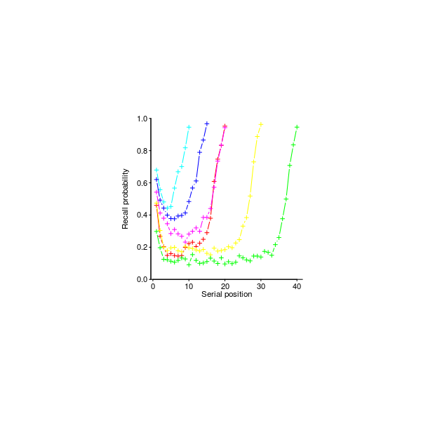
Figure 49. Probability of correct recall of words, by serial presentation order; for lists of length 10, 15 and 20 each word visible for 1, for lists of length 20, 30 and 40 each word visible for 2 seconds. Data from Murdoch Murdoch_62, via Brown Brown_07. Github--Local

Figure 50. Proportion of correctly recalled colored dot sequences of a given length, containing a given number of colors; lines are fitted regression models. Data kindly provided by Chekaf Chekaf_18. Github--Local

Figure 51. Hierarchical clustering of statement recall order, averaged over teachers and students; label names are: program_list-statementkind, where statementkind might be a function header, loop, etc. Data extracted from Adelson Adelson_81. Github--Local

Figure 52. Fraction of relearning time saved (normalised) after given interval since original learning; original Ebbinghaus study and three replications (with standard errors). Data from Murre et al Murre_15. Github--Local

Figure 53. Fraction of correct subject responses, with fitted bi-exponential model in red (blue and green lines are its two exponential components). Data from Rubin et al Rubin_99. Github--Local

Figure 54. Fraction of news items correctly recalled each day, after a given number of days since the event; Forced choice of one alternative from four, and Open requiring an answer with no suggestions provided. Data from Meeter et al Meeter_04. Github--Local

Figure 55. Time taken to solve the same jig-saw puzzle 35 times, followed by a two-week interval and then another 35 times, with power law and exponential fits. Data extracted from Alteneder Alteneder_35. Github--Local

Figure 56. Probability of assigning a stimulus to the correct category, where the category involved: height, position, and a combination of both height and position. Data from Kruschke Kruschke_93. Github--Local

Figure 57. Probability of assigning a stimulus to the correct category; learning the category, followed in block 23 by a change in the characteristics of the learned category. Data from Kruschke Kruschke_96. Github--Local

Figure 58. Completion times of eight solo developers for each implementation round. Data kindly provided by Lui Lui_06. Github--Local

Figure 59. Time taken, by the same person, to implement 12 algorithms from the Communications of the ACM (each colored line), with four iteration of the implementation process. Data from Zislis Zislis_73. Github--Local

Figure 60. Percentage occurrence of binary operator pairs (as a percentage of all such pairs) against the fraction of correct answers to questions about their precedence, red line is beta regression model. Data from Jones Jones_06a. Github--Local

Figure 61. Time taken by 24 subjects, classified by years of professional experience, to complete successive tasks. Data from Latorre Latorre_14. Github--Local

Figure 62. Elapsed months during which Asimov published a given number of books, with lines for two fitted regression models. Data from Ohlsson Ohlsson_92. Github--Local

Figure 63. Subjects' belief response curves when presented with evidence in the sequences: (upper) positive weak, then positive strong, (middle) negative weak then negative strong, (lower) positive then negative. Based on Hogarth et al Hogarth_92. Github--Local

Figure 64. Lines of code correctly recalled after a given number of 2-minute memorization sessions; actual program in upper plot, scrambled line order in lower plot. Data extracted from McKeithen et al McKeithen_81. Github--Local

Figure 65. One subject’s response time over successive blocks of command line trials and fitted loess (in green). Data kindly provided by Remington Remington_16. Github--Local

Figure 66. Country boundaries (green line) and town locations (red dots). Congruent: straight boundary aligned with question asked, incongruent: meandering boundary and locations sometimes inconsistent with question asked. Based on Stevens et al Stevens_78. Github--Local

Figure 67. Orthogonal representation of shape, color and size stimuli. Based on Shepard Shepard_61.

Figure 68. The six unique configurations of selecting four times from eight possibilities, i.e., it is not possible to rotate one configuration into another within these six configurations. Based on Shepard Shepard_61.

Figure 69. Percentage of correct category answers produced by one subject against boolean-complexity, broken down by number of positive cases needed to define the category used in the question (three colors). Data kindly provided by Feldman Feldman_00. Github--Local

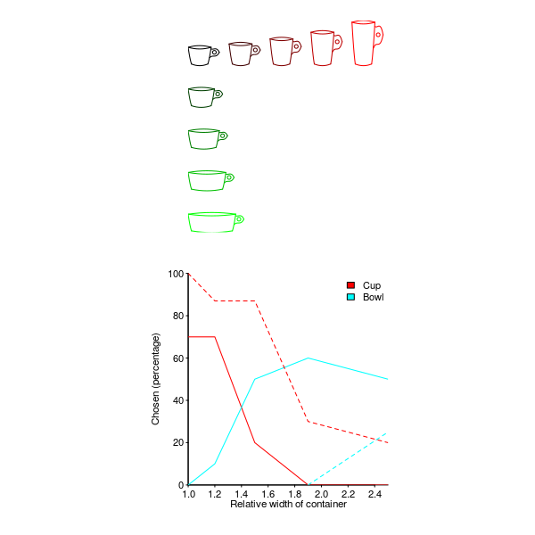
Figure 70. Cup- and bowl-like objects of various widths (ratios 1.2, 1.5, 1.9, and 2.5), and heights (ratios 1.2, 1.5, 1.9, and 2.4), with dashed lines showing neutral context and solid lines food context. The percentage of subjects who selected the term cup or bowl to describe the object they were shown (the paper did not explain why the figures do not sum to 100%, and color was not used in the original). Based on Labov Labov_73. Github--Local

Figure 71. A commercial event involving a buyer, seller, money and goods; as seen from the buy, sell, pay, or charge perspective. Based on Fillmore Fillmore_77. Github--Local

Figure 72. The four cards used in the Wason selection task. Based on Wason Wason_68. Github--Local

Figure 73. Example causal chains used Bramley Bramley_17. Github--Local

Figure 74. Average time (in milliseconds) taken for subjects to enumerate O’s in a background of X or Q distractors. Based on Trick and Pylyshyn Trick_93. Github--Local

Figure 75. Probability a subject will successfully distinguish a difference between the number of dots displayed, and a specified target number (x-axis is the difference between these two values). Data extracted from van Oeffelen et al van_Oeffelen_82. Github--Local

Figure 76. Line locations chosen for the numeric values seen by each of four subjects; color of fitted loess line changes at one million boundary. Data kindly provided by Landy Landy_17. Github--Local

Figure 77. Probability the rounded value given has actually been rounded, given an estimate of the likelihood of rounding, and the number of values likely to have been rounded; grey line shows 50% probability of rounding. Github--Local

Figure 78. Number of change requests having a given recorded time to decide whether change was needed, and time to implement. Data from Basili et al Basili_84. Github--Local

Figure 79. Min/max range of values (red/blue lines), and best value estimate (green circles), given by subjects interpreting the value likely expressed by statements containing “less than 100” and “more than 100”. Data kindly provided by Cummins Cummins_11. Github--Local

Figure 80. The cumulative probability of subjects expressing a given relative uncertainty, for numeric phrases using given hedge words. Data kindly provided by Ferson Ferson_15. Github--Local

Figure 81. Percentage of incorrect answers to arithmetic problems, given by Canadian and Chinese students, for each operand family value. Data kindly provided by LeFevre LeFevre_97. Github--Local

Figure 82. Estimated proportion (from survey results), and actual proportion of people in a population matching various demographics; line is a fitted regression having the form: $\mathit{lo} _\mathit{Estimated}\propto \gamma\times\mathit{lo} _\mathit{Actual} +(1-\gamma)\times\delta$, where $\gamma$ and $\delta$ are fitted constants; grey line shows estimated equals actual. Data from Landy et al Landy_18. Github--Local

Figure 83. Estimated probability (blue/green lines) of drawing a green ring by two subjects (upper: subject 10, session 8, lower: subject 7, session 8), with actual probability in red. Data from Khaw et al Khaw_17. Github--Local

Figure 84. Mean likelihood that a subject considered a dot of a given color to be blue, for the first/last 200 dots seen by two groups of subjects; lines are fitted logistic regression models. Data from Levari et al Levari_18. Github--Local

Figure 85. Fitted regression model for probability that a subject, who switched answer three times, switches their initial answer when told a given fraction of opposite responses were made by others (x-axis), broken down by confidence expressed in their answer (colored lines). Data kindly provided by Morgan Morgan_12. Github--Local

Figure 86. Each row shows a scaled version of the three stripes, along with actual lengths in inches, from which subjects were asked to select the longest. Based on Asch Asch_56. Github--Local

Figure 87. Risk neutral (green, $u(w)=w$), and example of risk loving (red, quadratic) and risk averse (blue, square-root) utility functions. Github--Local

Figure 88. Subjects' estimate of their ability (x-axis) to correctly answer a question and actual performance in answering on the left scale. The responses of a person with perfect self-knowledge is given by the green line. Data extracted from Lichtenstein et al Lichtenstein_77. Github--Local

Figure 89. Perceived present value (moving through time to the right) of two future rewards. Github--Local

Figure 90. Saving required (normalised), over a project having a given duration, before subjects would make a long term investment. Data from Becker et al Becker_19. Github--Local

Figure 91. Violin plots for actual time to complete problems for each of the 593 participants, sorted by mean solution time; colors to help break up the plots, and white line shows subject mean. Data from Nichols Nichols_19. Github--Local

Figure 92. Mean time for each of 36 subjects to choose between a given number of alternatives (upper), and accuracy rate for a given number of alternatives (lower), data has been jittered; lines are regression fits (yellow shows 95% confidence intervals), and color used for each subject sorted by performance on the two-choice case. Data from Hawkins et al Hawkins_12b. Github--Local

Figure 93. Percentage of employment by US industry sector 1850-2009. Data kindly provided by Kossik Kossik_11. Github--Local

Figure 94. Annual expenditure on custom, own account and prepackaged software by US business (plus lines) and the US federal and state governments (smooth lines). Data from Parker et al Parker_00. Github--Local

Figure 95. Number of people employed by major software companies. Data from Campbell-Kelly Campbell-Kelly_04. Github--Local

Figure 96. Company revenue ($millions) against total software development costs; line is a fitted regression model of the form: $\mathit{developmentCosts}\propto 0.19\mathit{Revenue}$. Data from Mulford et al Mulford_16. Github--Local

Figure 97. Average Return On Invested Capital of various U.S. industries between 1992-2006. Data from Porter Porter_08. Github--Local

Figure 98. Development cost (adjusted to 2018 dollars) of computer video games, whose cost was more than $50million. Data from Wikipedia Wiki_Games_18. Github--Local

Figure 99. Return/investment ratio needed to break-even, for Google and Mainframe application survival rate, having development/annual maintenance ratios of 5, 10 and 20; against payback period in years. Data from: mainframe Tamai Tamai_92, Google SaaS Ogden Ogden_20. Github--Local

Figure 100. Illustration of a drift diffusion process. Green lines show possible paths, red lines show bounds of diffusion and grey line shows drift with no diffusion component. Github--Local

Figure 101. Illustration of an Ornstein-Uhlenbeck process starting from zero and growing to its mean; green lines show various possible paths, red line is expected value, and blue lines one standard deviation. Github--Local

Figure 102. Example of a binomial model with three time-steps, given the probability $p$, of costs going up by $U$%, and the probability $1-p$, of costs going down by $D$%, at each time step, starting at $S$. Github--Local

Figure 103. Bug bounty payer (left) and payee (right) countries (total value $23,632,408). Data from hackerone Hackerone_17. Github--Local

Figure 104. Number of US patents granted in various areas. Data from Webb et al Webb_18. Github--Local

Figure 105. Normalised frequency of occurrences of code fragments containing a given number of lines; attributed to Stack Overflow answers, and unattributed close clones (a lognormal distribution is not sufficiently spikey to fit the data well). Data from Zhang et al Zhang_19. Github--Local

Figure 106. Cumulative percentage of files, from the top 10% largest Java projects, containing a given license (upper line is no license). Data from Vendome et al Vendome_17. Github--Local

Figure 107. Number of releases of packages containing a given number of licenses (a package has to contain a license to appear on CRAN). Data from Meloca et al Meloca_18. Github--Local

Figure 108. Survival curve of OSI licenses that have been listed on the approved license webpage, in days since 15 August 2000, with 95% confidence intervals. Data from opensource.org, via The Wayback Machine, web.archive.org. Github--Local

Figure 109. The cumulative number of hours worked per week by the 47 individuals involved with one avionics development project; dashed grey lines are straight lines fitted to three individuals. Data from Nichols et al Nichols_18. Github--Local

Figure 110. Number of proposals receiving a given number of mentions in emails; lines are a fitted regression models of the form: $\mathit{Mentions}\propto\mathit{Proposals}^{-a}$, where $a$ is $0.51$, $0.71$, and $0.81$. Data from Simcoe et al Simcoe_11. Github--Local

Figure 111. Percentage of passers-by looking up or stopping, as a function of group size; lines are fitted linear beta regression models. Data extracted from Milgram et al Milgram_69. Github--Local

Figure 112. Hours required to build a car radio after the production of a given number of radios, with break periods (shown in days above x-axis); lines are regression models fitted to each production period. Data extracted from Nembhard et al Nembhard_01. Github--Local

Figure 113. Man-hours required to build a particular kind of ship, at the Delta Shipbuilding yard, delivered on a given date (x-axis). Data from Thompson Thompson_07. Github--Local

Figure 114. Task rating given to members of successive generations of teams; lines are a regression model fitted to the one (red) and five (blue-green) write-up generation sequences. Data from Muthukrishna et al Muthukrishna_13. Github--Local

Figure 115. Ratio of actual to estimated hours of effort to enhance an existing product, for 25 versions of one application. Data from Huijgens et al Huijgens_16. Github--Local

Figure 116. Interval between product announcement date and its promised availability date, against interval between promised date and actual date the product became available; lines are a fitted regression model of the form: $\mathit{A{_}P}\propto e^{0.3-0.1\\\mathit{P{_}P} +0.8\\\sqrt{\mathit{P{_}P} }}$, and a loess fit. Data from Bayus et al Bayus_01. Github--Local

Figure 117. Mean number of deduction points specified by subjects told that a given percentage of subjects in a reference group cooperated; broken down by four subject response patterns. Data from Li et al Li_20. Github--Local

Figure 118. Percentage of individuals (x-axis) who correctly generated a solution, against mean response time, for 144 problems; colors denote time limits, and a sample of lines connecting performance pairs for the same program. Data from Bowden et al Bowden_03. Github--Local

Figure 119. Density plot of the difference between mean team mark and individual mark, broken down by team size. Data from Akdemir et al Akdemir_08. Github--Local

Figure 120. Average number of ideas produced by groups of a given size, at 5-minute interval elapsed time; dashed lines are nominal groups created by aggregating individual ideas. Data from Lewis Lewis_72. Github--Local

Figure 121. Time taken to publish an RFC having Standard or non-Standard status, for IETF committees having a given percentage of commercial membership (i.e., people wearing suits); lines are a fitted regression model with 95% confidence intervals (red), and a loess fit (blue/green). Data from Simcoe Simcoe_13. Github--Local

Figure 122. Percentage of developers, employed by given companies, working on OpenStack at the time of a release (x-axis). Data from Teixeira et al Teixeira_15. Github--Local

Figure 123. Survival curves of type I, II and III clones in the Linux high/medium/low level SCSI subsystems; dashed lines are 95% confidence intervals. Data from Wang Wang_12. Github--Local

Figure 124. Accounting practice for breaking down income from sales, and costs associated with major business activities. Github--Local

Figure 125. Average effort (in days) used to fix a fault experienced in a given phase (x-axis) caused by a mistake that had been introduced in an earlier phrase (colored lines), introduced in an earlier phase (total of 38,120 defects in projects at Hughes Aircraft). Data extracted from Willis et al Willis_98. Github--Local

Figure 126. Months of developer effort needed to produce systems containing a given number of lines of code, for various application domains; lines are quantile regression fits at 10 and 90%, for one application domain. Data from Gayek et al Gayek_04. Github--Local

Figure 127. Number of Apps in the Google playstore having a given number of releases; line is a fitted regression model of the form: $\mathit{Apps}\propto\mathit{Releases}^{-2.8}$. Data kindly provided by Li Li_18. Github--Local

Figure 128. Introductory price and performance (measured using wPrime32 benchmark; lower is better) of various Intel processors between 2003-2013. Data from Sun Sun_14. Github--Local

Figure 129. Vendor C and C++ compiler retail price (different line for each product), and upgrade prices (pluses) for products available under MS-DOS and Microsoft Windows between 1987 and 1998. Data kindly provided by Viard Viard_07. Github--Local

Figure 130. Examples of supply (lower) and demand (upper) curves. Github--Local

Figure 131. Rates at which product sales are made on Gumroad at various prices; lines join prices that differ in 1¢s;, e.g., $1.99 and $2. Data from Nichols Nichols_13. Github--Local

Figure 132. Sales of game software (solid lines) for the corresponding three major seventh generation hardware consoles (dotted lines). Data from VGChartz VGChartz_17. Github--Local

Figure 133. Growth of Github users during its first 58 months, with Bass models fitted to data up to a given number of months. Data from Irving Irving_16. Github--Local

Figure 134. Percentage of sales closed in a given week of a quarter, with average discount given. Data from Larkin Larkin_13. Github--Local

Figure 135. Facebook’s ARPU and cost of revenue per user. Data from Facebook’s 10-K filings Facebook_14Facebook_16. Github--Local

Figure 136. Top 100 software companies ranked by total revenue (in millions of dollars) and ranked by Software-as-a-Service revenue. Data from PwC PwC_13PwC_14PwC_16. Github--Local

Figure 137. Number of applications in the Android market and Amazon App Store, during 2012, containing a given number of advertising libraries (line is a fitted Negative Binomial distribution). Data from Shekhar et al Shekhar_12. Github--Local

Figure 138. Connections between the 164 companies that have Apps included in the Microsoft Office365 Marketplace (Microsoft not included); vertex size is an indicator of the number of Apps a company has in the Marketplace. Data kindly provided by van Angeren van_Angeren_16. Github--Local

Figure 139. Amount of memory installed on systems running a SPEC benchmark on a given date; lines are fitted quantile regression models dividing systems into 50% above/below, and 95% above with 5% below.. Data from SPEC SPEC_20 Github--Local

Figure 140. Yearly expenditure on punched cards, and tabulating equipment by the UK government. Data from Agar Agar_03. Github--Local

Figure 141. Total gigabytes of DRAM shipped world-wide in a given year, stratified by device capacity (in bits). Data from Victor et al Victor_02. Github--Local

Figure 142. Computer installation market share of IBM, and its top seven competitors (known at the time as the seven dwarfs; no data is available for 1969). Data from Brock Brock_75. Github--Local

Figure 143. Mobile phone operating system shipments, as percentage of total per year. Data from Reimer Reimer_12 (before 2007), and Gartner Gartner_17 (after 2006). Github--Local

Figure 144. Reported number of worldwide software industry mergers and acquisitions (M&A), per year. Data from Solganick Solganick_16. Github--Local

Figure 145. Average monthly donations received by 470 Github repositories using Patreon and OpenCollective. Data from Overney et al Overney_20. Github--Local

Figure 146. Monthly unit sales (in millions) of microprocessors having a given bus width. Data kindly provided by Turley Turley_02. Github--Local

Figure 147. Performance, in MIPS, against price of 106 computer systems available in 1981. Data from Ein-Dor Ein-Dor_85. Github--Local

Figure 148. Total sales of various kinds of processors. Data from Hilbert et al Hilbert_11. Github--Local

Figure 149. TSMC revenue from wafer production, as a percentage of total revenue, at various line widths. Data from TSMC TSMC_17. Github--Local

Figure 150. Survival curve for GCC’s support for distinct cpus and non-processor specific compile-time options; with 95% confidence intervals. Data extracted from gcc website GCC_opts_19. Github--Local

Figure 151. Maximum speed achieved by vehicles over the surface of the Earth, and in the air, over time. Data from Lienhard Lienhard_06. Github--Local

Figure 152. Number of transistors, frequency and SPEC performance of cpus when first launched. Data from Danowitz et al Danowitz_12. Github--Local

Figure 153. Number of major forks of projects per year, identified using Wikipedia during August 2011. Data from Robles et al Robles_12b. Github--Local

Figure 154. Phylogenetic tree of Debian derived distributions, based on which of 50,708 packages are included in each distribution. Data from Keil et al Keil_16. Github--Local

Figure 155. Percentage of code ported from NetBSD to various versions of OpenBSD, broken down by version of NetBSD in which it first occurred (denoted by incrementally changing color). Data kindly provided by Ray Ray_13. Github--Local

Figure 156. Number of websites running a given version of PHP on the first day of February, 2016 and 2017, ordered by PHP version number. Data kindly provided by Ruohonen Ruohonen_17. Github--Local

Figure 157. Decade in which newly designed US Air Force aircraft first flew, with colors indicating current operational status. Data from Echbeth el at Eckbreth_11. Github--Local

Figure 158. Mean age of installed mainframe computers, 1968-1983. Data from Greenstein Greenstein_94. Github--Local

Figure 159. Survival curve of Linux distributions derived from five widely-used parent distributions (identified in legend). Data from Lundqvist et al Lundqvist_12. Github--Local

Figure 160. Percentage share of Android market, of a given release, by days since its launch. Data from Villard Villard_15. Github--Local

Figure 161. Number of software systems surviving for a given number of days and fitted regression models: Japanese mainframe software (red), Google software-as-a-service (blue; 202 systems as of October 2020). Data from: mainframe Tamai Tamai_92, Google’s SaaS Ogden Ogden_20. Github--Local

Figure 162. Size at foundation and lifetime of 32 secular and 19 religious 19th century American utopian communities; lines are fitted loess regression. Data from Dunbar et al Dunbar_18. Github--Local

Figure 163. Number of US companies manufacturing automobiles and PCs, over the first 30-years of each industry. Data extracted from Mazzucato Mazzucato_01. Github--Local

Figure 164. Retail prices of Model T Fords and sales volume. Data from Hounshell Hounshell_84. Github--Local

Figure 165. Example showing difference in number of customers using two products. Github--Local

Figure 166. Number of programs in the Ubuntu AMD64 distribution shipped using a given security hardening technique (Total ELF is the number of ELF executables). Data from Cook Cook_19. Github--Local

Figure 167. Number of process model change requests made in three years of a banking Customer registration project. Data kindly provided by Branco Branco_12. Github--Local

Figure 168. Growth in the number of projects within the Apache ecosystem, along with the amount of contained code. Data from Bavota et al Bavota_13. Github--Local

Figure 169. Percentage overlap of developers contributing, during 2013, to both of each pair of 147 Apache projects. Data kindly provided by Panichella Bavota_15. Github--Local

Figure 170. Total computer systems purchased and rented by the US Federal Government in the respective fiscal years ending June 30. Data from US Government General Accounting Office Staats_71. Github--Local

Figure 171. Total U.S. revenue from sale of computer systems and data processing service industry revenue. Data from Phister Phister_79 table II.1.20 and II.1.26. Github--Local

Figure 172. Total yearly spend on their own software by the 21 industry sectors in the UK, reported by companies as fixed-assets. Data from UK Office for National Statistics Off_Nat_Stat_17. Github--Local

Figure 173. Cumulative number of software requirements added, modified and deleted, over successive releases, to the 11,000+ requirements present in release 4.0.0. Data kindly provided by Motta Motta_16. Github--Local

Figure 174. Typical memory capacity against cost of 167 different computer systems from 1970 to 1978; fitted regression lines are for 1971, 1974 and 1977. Data from Cale Cale_79. Github--Local

Figure 175. Estimated number of comments written in German, in the LibreOffice source code. Data from Meeks Meeks_17. Github--Local

Figure 176. Number of new UK companies registered each month, whose SIC description includes the word software (45,422 entries) or computer (18,001 entries). Data extracted from OpenCorporates OpenCorporates_15. Github--Local

Figure 177. Connections between companies in a Dutch software business network. Data kindly provided by Crooymans Crooymans_15. Github--Local

Figure 178. Number of people employed in the 12 computer occupation codes assigned by the U.S. Census Bureau during 2014, stratified by ages bands (main peak is the total, “Software developers, applications and system software” is the largest single percentage; see code for the identity of other occupation codes). Data from Beckhusen Beckhusen_16. Github--Local

Figure 179. The job categories contained within the seven career paths in which people spent at least five years working in technical IT role. Data from Joseph et al Joseph_12. Github--Local

Figure 180. Sorted list of total amount awarded by bug bounties to individual researchers, based on two datasets downloaded from HackerOne. Data from Zhao et al Zhao_15 and Maillart et al Maillart_17. Github--Local

Figure 181. Daily minutes spent using an App, from Apple’s AppStore (data from 2009); lines are a loess fit. Data extracted from Ansar Ansar_09. Github--Local

Figure 182. Size of 40 operating systems (Kbytes, measured in 1975) capable of controlling a given number of unique devices; line is a quadratic regression fit. Data from Elci Elci_75. Github--Local

Figure 183. Number of pdf files created using a given version of the portable document format appearing on sites having a .uk web address between 1996 and 2010. Data from Jackson Jackson_12. Github--Local

Figure 184. Ratio of development costs to average annual maintenance costs (over 5-years) for 158 IBM software systems sorted by size; curve is a beta distribution fitted to the data (in red). Data from Dunn Dunn_11. Github--Local

Figure 185. Number of Unix processes executing for a given number of seconds, on a 1995 era computer. Data from Harchol-Balter et al Harchol-Balter_95. Github--Local

Figure 186. Total instructions contained in the software shipped with various models of IBM computer, plus Datatron from Burroughs; line is a fitted regression of the form: $\mathit{Instructions}\propto e^{0.4\mathit{Year} }$. Data extracted from Naur et al Naur_69. Github--Local

Figure 187. Number of new programming languages, per year, described in a published paper. Data from Pigott et al Pigott_15. Github--Local

Figure 188. Lines of code written in the 32 programming languages appearing in the source code of the 13 major Debian releases between 1998 and 2019. Data from the Debsources developers Debsources_dev_19. Github--Local

Figure 189. Monthly labor market slack (i.e., applications per days vacancy listed) for jobs whose description included a particular keyword (see legend). Data from Davis et al Davis_17. Github--Local

Figure 190. Number of monthly developer job related tweets specifying a given language. Data kindly provided by Destefanis Destefanis_14. Github--Local

Figure 191. Normalised percentage of 34 language tags associated with questions appearing on Stack Overflow in each month. Data extracted from Stack Overflow website SO_trends_19. Github--Local

Figure 192. Percentage of universities reporting the first language used to teach computer science majors. Data from Reid, via the Wayback Machine, Reid_02. Github--Local

Figure 193. Cumulative number of Github projects that can be built as more gcc built-ins are implemented. Data from Rigger et al Rigger_19. Github--Local

Figure 194. Number of Android/Ubuntu (1.1 million apps)/(71,199 packages) linking to a given POSIX function (sorted into rank order). Data from Atlidakis et al Atlidakis_16. Github--Local

Figure 195. Percentage of packages referencing a particular API provided by a given service (sorted in rank order); grey lines are a fitted power law and exponential, to ioctl and libc respectively. Data from Tsai et al Tsai_16. Github--Local

Figure 196. Survival curve of packages included in 10 official Debian releases, and inclusion of the same release of a package; dashed lines are 95% confidence intervals. Data from Caneill et al Caneill_14. Github--Local

Figure 197. Number of packages in three widely used &R; repositories (during 2015), overlapping regions show packages appearing in multiple repositories (areas not to scale). Data from Decan et al Decan_15. Github--Local

Figure 198. Survival curves for Debian package lifetime and interval before a package contains its first dependency conflict; dashed lines are 95% confidence intervals. Data from Drobisz et al Drobisz_15. Github--Local

Figure 199. Number of Android APIs surviving a given number of releases (measured over 17 releases), with fitted regression lines. Data from Li et al Li_16. Github--Local

Figure 200. Phylogenetic tree of 1,663 cryptocurrency implementations, based on the fraction of shared source code files. Data kindly provided by Yousaf Reibel_18. Github--Local

Figure 201. Number of gcc compiler options, for all supported versions, relating to languages and the process of building an executable program. Data extracted from gcc website GCC_opts_19. Github--Local

Figure 202. Words in Intel x86 architecture manuals, and code-points in Unicode Standard over time. Data for Intel x86 manual kindly provided by Baumann Baumann_16. Github--Local

Figure 203. Number of projects having a given duration (upper; 2,992 projects), delivered containing a given number of SLOC (middle; 1,859 projects), and using a given percentage of out-sourced effort (lower; 1,267 projects). Data extracted from Akita et al Akita_12. Github--Local

Figure 204. Firm bid price (in euros) against schedule estimate (in days), received from 14 companies, for the same tender specification. Data from Anda et al Anda_09. Github--Local

Figure 205. Annual development cost and lines of code delivered to the US Air Force between 1960 and 1986. Data extracted from NeSmith NeSmith_86. Github--Local

Figure 206. Distribution of effort (person hours) during the development of four engine control system projects (various colors), plus non-project work (blue) and holidays (purple’ish, at top), at Rolls-Royce. Data extracted from Powell Powell_01. Github--Local

Figure 207. Percentage profit/loss on 145 fixed-price software development contracts. Data extracted from Coombs Coombs_03. Github--Local

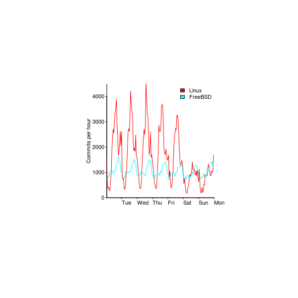
Figure 208. Commits within a particular hour and day of week for Linux and FreeBSD. Data from Eyolfson et al Eyolfson_11. Github--Local

Figure 209. Survival rate of 214 projects, by development stage, with 95% confidence intervals. Data from McManus et al McManus_07. Github--Local

Figure 210. Estimated and Actual effort for internal and external projects, lines are fitted regression models; both lines are fitted regression models of the form: $\mathit{Actual}\propto \mathit{Estimate}^a$, where $a$ takes the value 0.9 or 1.1. Data from Moløkken-Østvold et al Molokken_Ostvold_04. Github--Local

Figure 211. Bids made by 19 estimators from the same company (divided by grey line into the two experimental groups). Data from Jørgensen et al Jorgensen_04c. Github--Local

Figure 212. Project effort, in thousands of hours, against percentage of management time, broken down by contract type; both lines are fitted logistic equations with maximums of 12% and 16%. Data extracted from Ahonen Ahonen_15. Github--Local

Figure 213. Mean number of years experience of each team against estimated project code, with fitted regression models; broken down by teams containing one or more members who have had similar project experience, or not. Data from Mcdonald Mcdonald_05. Github--Local

Figure 214. Estimated and actual project implementation effort; 49 web implementation tasks (blue), and 145 tasks performed by an outsourcing company (red). Data from Jørgensen Jorgensen_04b and Kitchenham et al Kitchenham_02. Github--Local

Figure 215. Two estimates (in work hours), made by seven subjects, for each of six tasks. Data from Grimstad et al Grimstad_07. Github--Local

Figure 216. Mean rate of construction, in meters per year, of skyscrapers taller than 150 m (error bars show standard deviation). Data kindly provided by Recon Recon_18. Github--Local

Figure 217. Estimates given by three groups of subjects after seeing a statement by a middle manager containing an estimate (2 months or 20 months) or no estimate (control); sorted to highlight distribution. Data from Aranda Aranda_05. Github--Local

Figure 218. Density plot of the investment, by 2,570 projects, of a given fraction of total effort in a given project phase. Data kindly provided by Wang Wang_17. Github--Local

Figure 219. Number of tasks having a given estimate, and a given actual implementation time. Data from Jones et al Jones_19a. Github--Local

Figure 220. Estimated project cost from 12 estimating models. Data from Mohanty Mohanty_81. Github--Local

Figure 221. Elapsed weeks (x-axis) against effort in man-hours per week (y-axis) for a project, plus three fitted curves. Data extracted from Basili et al Basili_81. Github--Local

Figure 222. Function points and corresponding normalised costs for 149 projects from one large institution; line is a fitted regression model of the form: $\mathit{Cost}\propto \mathit{Function{_}Points}^{0.75}$. Data extracted from Kampstra el al Kampstra_09b. Github--Local

Figure 223. Cost per requirement, function point and story point for two projects, over 13 monthly releases. Data from Huijgens Huijgens_13. Github--Local

Figure 224. Estimated effort to implement 24 story-points and corresponding COSMIC function point; line is a fitted regression model of the form: $\mathit{CosmicFP}\propto \mathit{storyPoint}^{0.6}$, with 95% confidence intervals. Data from Commeyne et al Commeyne_16. Github--Local

Figure 225. Mean LOC against standard deviation of LOC, for multiple implementations of seven distinct problems; line is a fitted regression model of the form: $\mathit{Standard{_}deviation}\propto \mathit{SLOC}$. Data from: Anda et al Anda_09, Jørgensen Jorgensen_16b, Lauterbach Lauterbach_87, McAllister et al McAllister_89, Selby et al Selby_85, Shimasaki et al Shimasaki_80, van der Meulen van_der_Meulen_07. Github--Local

Figure 226. Mean and median effort (thousand hours) for projects having a given elapsed time; both lines are a fitted regression model of the form: $\mathit{Effort}\propto \mathit{Duration}^2$. Data from Wang et al Wang_17. Github--Local

Figure 227. IBM’s profit margin on all System 360s sold in 1966, by system memory capacity in kilobytes; monthly rental cost during 1967 in parentheses. Data from DeLamarter DeLamarter_88. Github--Local

Figure 228. COSMIC function-points and compiled size (in kilobytes) of components in four different ECU modules; lines show fitted regression model. Data from Lind et al Lind_12. Github--Local

Figure 229. Number of requirements and corresponding lines of manually created source code, for each team (colors denote language used). Data from Prechelt Prechelt_07 Github--Local

Figure 230. Initial implementation schedule, with employee number(s) given for each task (percentage given when not 100%) for a project. Data from Ge et al Ge_16. Github--Local

Figure 231. Evolution of the estimated cost of developing a bespoke software system, as implementation progressed; over time the estimated costs shift between the Prime contractor and its two subcontractors. Data from Yu Yu_03. Github--Local

Figure 232. Phase during which work on a given activity of development was actually performed, average percentages over 13 projects. Data from Zelkowitz Zelkowitz_87. Github--Local

Figure 233. Percentage distribution of effort time (red) and schedule time (blue) across design/coding/testing for 38 NASA projects. Data from Condon et al Condon_93. Github--Local

Figure 234. Percentage distribution of effort across design/coding/testing for 10 ICL projects (red), 11 BT projects (green), 11 space projects (blue) and 12 defense projects (purple). Data from Kitchenham et al Kitchenham_85 and Graver et al Graver_77. Github--Local

Figure 235. Effort, in person hours per month, used in the implementation of the five components making up the PAVE PAWS project (grey line shows total effort). Data extracted from Curtis et al Curtis_80. Github--Local

Figure 236. Percentage of actual project duration elapsed at the time 882 schedule estimates were made, during 121 projects, against estimated/actual time ratio (y-axis has a log scale; boundary maximum in red). Data kindly provided by Little Little_06. Github--Local

Figure 237. Initial estimated project duration against number of schedule estimates made before completion, for 121 projects; line is a loess fit. Data kindly provided by Little Little_06. Github--Local

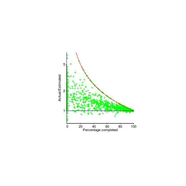
Figure 238. Percentage change in 882 estimated delivery dates, announced at a given percentage of the estimated elapsed time of the corresponding project, for 121 projects (red is a loess fit); blue line is a density plot of percentage estimated duration when the estimate was made. Data kindly provided by Little Little_06. Github--Local

Figure 239. Percentage of work packages having a given lead time that are completed within a given duration; colored lines are work packages having the same estimated lead time. Data extracted from van Oorschot et al van_Oorschot_05. Github--Local

Figure 240. Number of Marathon competitors finishing in a given number of minutes (250,000 runner sample size). Data from Allen et al Allen_17. Github--Local

Figure 241. Aggregated salience of each stakeholder, calculated using the pagerank of the stakeholders in the network created from the Open (red) and Closed (blue) stakeholder responses (values for each have been sorted). Data from Lim Lim_10. Github--Local

Figure 242. Average value assigned to requirements (red) and one standard deviation bounds (blue) based on omitting one stakeholder’s priority value list. Data from Regnell et al Regnell_01. Github--Local

Figure 243. Number of features whose implementation took a given number of elapsed workdays; red first 650-days, blue post 650-days, green lines are fitted zero-truncated negative binomial distributions. Data kindly supplied by 7Digital 7Digital_12. Github--Local

Figure 244. Average number of days taken to implement a feature, over time; smoothed using a 25-day rolling mean. Data kindly supplied by 7Digital 7Digital_12. Github--Local

Figure 245. Number of feature developments started on a given work day (red new features, green bugs fixes, blue ratio of two values; 25-day rolling mean). Data kindly supplied by 7Digital 7Digital_12. Github--Local

Figure 246. Number of tasks having a given duration, in elapsed working days, between estimating/starting (blue), and starting/completing (red). Data from Jones et al Jones_19a. Github--Local

Figure 247. Total number of story points and hours worked during each sprint of project P1. Data kindly provided by Vetrò Vetro_18. Github--Local

Figure 248. Violin plots of benchmark times for a sample of 33 commits to SAX builder (average of 7,357 measurements per commit). Data from Horký Horky_18. Github--Local

Figure 249. Number of projects on Github (out of 2,923) having a given number of branches; the line is a fitted regression model of the form: $\mathit{projects}\propto \mathit{branches}^{-2}$. Data from Zou et al Zou_19. Github--Local

Figure 250. Number of optional features selected by a given number of flags. Data kindly provided by Berger Berger_12. Github--Local

Figure 251. Number of identifiers renamed, each month, in the source of Eclipse-JDT; version released on given date shown. Data from Eshkevari et al Eshkevari_11. Github--Local

Figure 252. Percentage of commits outstanding against percentage the time remaining before deployment, for 18 releases; blue/green transition is the feature freeze date, red line shows a constant commit rate. Data kindly provided by Laukkanen Laukkanen_17. Github--Local

Figure 253. Number of failed jobs in Travis CI builds involving a given number of jobs (points have been jittered); line is a loess fit. Data from Gallaba et al Gallaba_18. Github--Local

Figure 254. Survival curve of IT outsourcing suppliers continuing to work for 2,382 Credit Unions. Data kindly provided by Peukert Peukert_10. Github--Local

Figure 255. Average number of hours worked per month (by an individual), with standard deviation, for two projects staffed by 1,657 and 834 people; two red lines and corresponding error bars offset either side of month value. Data kindly provided by Bao Bao_17. Github--Local

Figure 256. Number of projects making use of a given number of different languages in a sample of 100,000 GitHub project. Data kindly provided by Bissyande Bissyande_13. Github--Local

Figure 257. Number of tasks worked on by a given number of developers. Data from Nichols et al Nichols_18 and Jones et al Jones_19a. Github--Local

Figure 258. Number of days before planned product ship date, against number of full time engineers, for each of the 63 months since the project started (numbers show months since project started). Data from Jackson Jackson_89. Github--Local

Figure 259. Effective rate of production of a team containing a given number of people, with communication overhead $t_0=t_1=0.1$, and various distributions of percentage communication time; black line is zero communications overhead. Github--Local

Figure 260. Time taken by groups of different sizes to manually assembly a product, over multiple trials; lines are fitted regression models of the form: $\mathit{Time}\propto ~ \frac{0.5-0.2\log(\mathit{Repetitions} )}{\mathit{Group{_}size} }-0.1\log(\mathit{Repetitions} )$. Data kindly provided by Peltokorpi et al Peltokorpi_19. Github--Local

Figure 261. Time-line of first @word usage, ordered on y-axis by date of first appearance; legend shows @words with more than 500 occurrences. Data from Jones et al Jones_19c. Github--Local

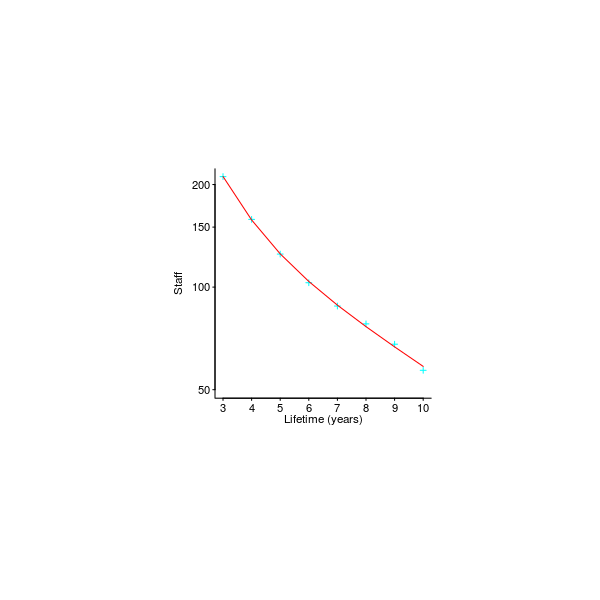
Figure 262. Average number of staff required to support renewal of code having a given average lifetime (green); blue/red lines show fitted biexponential regression model. Data extracted from Elliott Elliott_77. Github--Local

Figure 263. Age of systems, developed using one of two methodologies, and corresponding monthly maintenance effort, lines are loess regression fits. Data extracted from Dekleva Dekleva_92. Github--Local

Figure 264. Number of lines of code in a release (x-axis) originally added in a given release (colored lines). Data kindly provided by Ozment Ozment_06. Github--Local

Figure 265. Growth of PC-Lint, over 11 major releases in 28 years, of messages supported, command line options, kilo-words in product manual, and thousands of lines of code in the product. Data kindly provided by Gimpel Gimpel_14. Github--Local

Figure 266. Percentage of requirements added/deleted/modified for eight features (colored lines) of a product over 22 releases. Data extracted from Felici Felici_04. Github--Local

Figure 267. Ternary plot showing developers' estimated and actual percentage time breakdown performing adaptive, corrective and perfective work accumulated over 1,294 maintenance tasks; size of accumulation denoted by circle size. Data from Hatton Hatton_07. Github--Local

Figure 268. Percentage of patches submitted to WebKit (34,535 in total) transitioning between various stages of code review. Data from Baysal et al Baysal_13. Github--Local

Figure 269. Density plot of interval between a patch passing review and being accepted by a maintainer, and interval between a maintainer pushing the patch to Linus Torvalds, and it being accepted into the blessed mainline (only patches accepted by Torvalds included). Data from Jiang et al Jiang_13. Github--Local

Figure 270. Evolution of the number of tables in the Mediawiki and Ensembl project database schema. Data from Skoulis Skoulis_13. Github--Local

Figure 271. Survival curve for tables in Wikimedia and Ensembl database schema, with 95% confidence intervals. Data from Skoulis Skoulis_13. Github--Local

Figure 272. Survival curve for year of last modification of database programs, i.e., years before they stopped being changed, with 95% confidence intervals. Data from Blum Blum_89. Github--Local

Figure 273. Survival rate of reported fault experiences in Linux device drivers and the other Linux subsystems. Data from Palix et al Palix_10b. Github--Local

Figure 274. Flow of updates between participants in one Android ecosystem; number of each kind of member given in brackets, number of updates shipped on edges (in blue). Data from Thomas Thomas_15. Github--Local

Figure 275. Accuracy of the value returned by the $\cos$ instruction on an Intel Core i7, for 52,521 argument values close to $\frac{\pi}2$. Data kindly provided by Duplichan Duplichan_13. Github--Local

Figure 276. Reported faults against number of installations (upper) and age (lower). Data from the "wheezy" Debian release UDD_14. Github--Local

Figure 277. Duplicates of Eclipse fault report 4671 (report 6325 was finally chosen as the master report); arrows point to report marked as duplicate of an earlier report. Data from Sadat et al Sadat_17. Github--Local

Figure 278. Six fault reports (red), their associated bug fixing commits (blue), and subsequent commits to fix mistakes introduced by the earlier commit (blue). Data from Xiao et al Xiao_20. Github--Local

Figure 279. Mean percentage likelihood of (translated) statements containing a probabilistic term; one colored line per country. Data from Budescu et al Budescu_14. Github--Local

Figure 280. Subjects' perceived change in the magnitude of a quantity, when the given gradable size adjective is present. Data from Sharp et al Sharp_18. Github--Local

Figure 281. Survival curves of the two most common warnings reported by Splint in Samba and Squid, where survival was driven by code changes and not fixing a reported fault; with 95% confidence intervals. Data from De Penta et al Di_penta_09. Github--Local

Figure 282. Cumulative number of class III (high-risk) medical devices, containing software in their product summary, achieving premarket approval from the FDA. Data from FDA FDA_19. Github--Local

Figure 283. Value of bounties offered for 2,816 tasks addressing specified open issues of a Github project; pledges stratified by status of person reporting the pledge issue. Data from Zhou et al Zhou_19. Github--Local

Figure 284. Number of incidents reported for each of 800 applications installed on over 120,000 desktop machines; line is fitted regression model. Data from Lucente Lucente_15. Github--Local

Figure 285. Number of exceptions experienced per day against number of new users of the application, for one application prior to its general release; line is a fitted regression model of the form: $\mathit{Exceptions}\propto \mathit{newUserUses}^{0.8}$. Data from Dey et al Dey_20. Github--Local

Figure 286. Number of accesses to memory address blocks, per 100,000 instructions, when executing gzip on two different input files. Data from Brigham Young Brigham_Young via Feitelson. Github--Local

Figure 287. Transition counts of five distinct fault experiences in 50 runs of program A2; nodes labeled with each fault experienced up to that point. Data from Nagel et al Nagel_82. Github--Local

Figure 288. Number of input cases processed before a particular fault was experienced by program A2; the list is sorted for each distinct fault. Data from Nagel et al Nagel_82. Github--Local

Figure 289. Number of input cases processed by two implementations before a fault was experienced, with four replications (each a different color); grey lines are a regression fit for one implementation. Data from Dunham et al Dunham_86. Github--Local

Figure 290. Number of input cases processed by program AT1 before a given fault was experienced, during 25 replications. Data from Dunham et al Dunham_86. Github--Local

Figure 291. Faults experienced against hours of testing, for four releases of a product. Data from Wood Wood_96. Github--Local

Figure 292. Time taken to encounter a thread safety violation in 22 Java classes, violin plots for 10 runs of each class. Data kindly supplied by Pradel Pradel_12. Github--Local

Figure 293. Percentage of fault experiences having a given mean time to first experience (in months, over all installations of a product), for nine products. Data from Adams Adams_84. Github--Local

Figure 294. Number of times the same fault was experienced in one program, crashes traced to the same program location; with fitted biexponential equation (green line; red/blue lines the two components). Data kindly provided by Zhao Zhao_16. Github--Local

Figure 295. Violin plots of likelihood (local y-axis) that an add-one perturbation at a (normalised) program location will not change the output behavior. Data from Danglot et al Danglot_18. Github--Local

Figure 296. Predicted growth, with 95% confidence intervals, in the number of new crash fault experiences in the 2003, 2007 and 2010 releases of Microsoft Office. Data from Kaminsky et al Kaminsky_11. Github--Local

Figure 297. Number of crashes traced to the same executable location (sorted by number of crashes), in the 2003, 2007 and 2010 releases of Microsoft Office; lines are fitted biexponential regression models. Data from Kaminsky et al Kaminsky_11. Github--Local

Figure 298. Number of occurrences of the same mistake responsible for a reported fault in GCC, with fitted biexponential regression model, and component exponentials. Data from Sun et al Sun_16. Github--Local

Figure 299. Number of instances of the same reported fault in KDE, with fitted triexponential regression model. Data from Sadat et al Sadat_17. Github--Local

Figure 300. Lines of source in early versions of Firefox, broken down by the version in which it first appears. Data extracted from Massacci et al Massacci_11. Github--Local

Figure 301. Market share of Firefox versions between official release and end-of-support (left of grey line are estimates, right are measurements). Data from Jones Jones_13. Github--Local

Figure 302. End-user usage of code originally written for Firefox version 1.0, by major released versions (in units of LOC*Users); red points show sum over all versions. Based on data from Jones Jones_13 and extracted from Massacci et al Massacci_11. Github--Local

Figure 303. Total number of implementations in each of 36 equivalence classes, plus both first and last competitor submissions. Data from van der Meulen et al van_der_Meulen_04. Github--Local

Figure 304. Violin plot of the time taken to response to a question about a requirement, for nine quantifiers paired by affirmative/negative. Data from Winter et al Winter_20. Github--Local

Figure 305. Cumulative number of potential defects logged against the POSIX standard, by defect classification. Data kindly provided by Josey OpenGroup_17. Github--Local

Figure 306. Ranked occurrences of compiler messages generated by student submitted Java and Python programs. Data from Pritchard Pritchard_15. Github--Local

Figure 307. Fraction of mutated programs, in various languages, that successfully compiled/executed/produced the same output. Data from Spinellis et al Spinellis_12. Github--Local

Figure 308. Number of fault reports whose fixes involved a given number of files, modules or lines in a sample of 290 faults in AspectJ; lines are fitted power laws. Data from Lucia Lucia_14. Github--Local

Figure 309. Normalized number of commits (i.e., each maximum is 100), made to address fault reports, involving a given number of files in five software systems; grey line is representative of regression models fitted to each project, and has the form: $\mathit{Commits}\propto \mathit{Files}^{-2.1}$. Data from Zhong et al Zhong_15 via M. Monperrus. Github--Local

Figure 310. Percentage of insertions/modifications of a given number of lines resulting in a reported fault; lines are fitted beta regression models of the form: $\mathit{percent{_}faultReports}\propto \log(\mathit{Lines} )$. Data from Purushothaman et al Purushothaman_05. Github--Local

Figure 311. Survival curve (with 95% confidence bounds) of time to fix vulnerabilities reported in npm packages (Base) and time to update a package dependency (Depend) to a corrected version (i.e., not containing the reported vulnerability); for vulnerabilities with severity high and medium. Data from Decan et al Decan_18. Github--Local

Figure 312. Number of bit-flips in SRAM fabricated using various processes, with devices on top of, or under a mountain in the French Alps. Data kindly provided by Autran Autran_12. Github--Local

Figure 313. For systems 2 and 18, number of uptime intervals, binned into 10 hour intervals, red lines are both fitted negative binomial distributions. Data from Los Alamos National Lab (LANL). Github--Local

Figure 314. Fault slip throughs for a development project at Ericsson; y-axis lists phase when fault could have been detected, x-axis phase when fault was found. Data from Hribar et al Hribar_08. Github--Local

Figure 315. Reported time taken to correct 7,095 mistakes (in one project), broken down by phase the mistake was introduced/corrected (y-axis), against number of phases between introduction/correction (x-axis); lines are fitted regression models of the form: $\mathit{Fix{_}time}\propto e^{\sqrt{\mathit{phase{_}sep} }}$, with fix times less than 1, 5 and 10-minutes excluded. Data from Nichols et al Nichols_18. Github--Local

Figure 316. Number of vulnerabilities found using black-box testing, and manual code review of nine implementations of the same specification. Data from Finifter Finifter_13b. Github--Local

Figure 317. Fraction of usability problems found by a given number of subjects/evaluations in 12 system evaluations; lines are fitted regression model for each system. Data extracted from Nielsen et al Nielsen_93. Github--Local

Figure 318. Probability (y-axis) of a given number of issues being found (x-axis), by a review group containing a given number of people (colored lines). Data from Lewis Lewis_01. Github--Local

Figure 319. Number of faults experienced per unit of testing effort, over a given number of weeks (each normalised to sum to 100). Data from Stikkel Stikkel_06. Github--Local

Figure 320. Statement coverage achieved by the respective program’s test suite (data on the sixth program was not usable). Data from Marinescu et al Marinescu_14. Github--Local

Figure 321. Violin plots of percentage of regular expression components having a given coverage, (measured using the nodes and edges of the DFA representation of the regular expression, broken down by the match failing/succeeding) for 15,096 regular expressions, when passed the corresponding project test input strings. Data kindly provided by Wang Wang_18b. Github--Local

Figure 322. Percentage of known faults experienced for tests involving a given number of combinations of factors (x-axis), for ten programs. Data from Kuhn et al Kuhn_17. Github--Local

Figure 323. Statement coverage against branch coverage for 300 or so Java projects; colored lines are fitted regression models for three program sizes (see legend), equal value line in grey. Data from Gopinath et al Gopinath_14. Github--Local

Figure 324. Number of statements executed along error and non-error paths within a function (top), and density plots of the number of statements along error and non-error paths. Data kindly provided by Kang Kang_16. Github--Local

Figure 325. Basic-block coverage against branch coverage for a 35 KLOC program; lines are a regression fit (red) and $\mathit{Decision} =\mathit{Block}$ (grey). Data from Gokhale et al Gokhale_06. Github--Local

Figure 326. Fraction of basic-blocks executed by a given number of tests, for 20 implementations using three test suites. . Data from McAllister et al McAllister_89. Github--Local

Figure 327. Statement coverage against mutants killed for 300 or so Java projects; colored lines are fitted regression models for three program sizes, equal value line in grey. Data from Gopinath et al Gopinath_14. Github--Local

Figure 328. Unit cost of a missile, developed for the US military, against the number of development test flights carried out, with fitted power law. Data extracted from Augustine Augustine_97. Github--Local

Figure 329. Composite image of brain areas active when 30 subjects categorized Java code snippets; colored scale based on t-value of the decoding accuracy of source code categories from the MRI signals. Image from Ikutani et al Ikutani_20.

Figure 330. Lines of code in published implementations of the collected algorithms of the Transactions on Mathematical Software; line is a fitted regression of the form: $\mathit{LOC}\propto e^{0.0003\mathit{Day} }$. Data extracted by your author. Github--Local

Figure 331. Fraction of files in high-level categories for 23,715 repositories containing a given number of files (averaged over all repositories containing a given number of files). Data from Pfeiffer Pfeiffer_20. Github--Local

Figure 332. Number of source files, methods, and lines of code within methods, contained in each of 13,103 Java projects; lines are kernel density plots. Data kindly provided by Landman Landman_16. Github--Local

Figure 333. Number of files and lines of code in 3,782 projects hosted on Sourceforge. Data from Herraiz Herraiz_08. Github--Local

Figure 334. Percentage of call instructions contained in code generated from the same C source, against call execution percentage for various processors; grey line is fitted regression model. Data from Davidson et al Davidson_89b. Github--Local

Figure 335. Time to compile, using -O3 optimization, each of 71,200 function (in the SPEC benchmark) containing a given number of LLVM instructions; line shows fitted regression model for one trend in the data. Data kindly provided by Auler Auler_13. Github--Local

Figure 336. Probability that a worker having a given ability (x-axis) will correctly answer a given question (numbered colored lines); fitted using item response theory. Data from Chapman et al Chapman_17. Github--Local

Figure 337. Number of for-loops, in C source, whose enclosed compound-statement contained basic blocks nested to a given depth; with fitted exponential (upper) and power law (lower). Data kindly provided by Pani Pani_13. Github--Local

Figure 338. Lines of code, Halstead’s volume and McCabe’s cyclomatic complexity of the 62,365 C functions containing at least 10 lines, in Linux version 2.6.9; fitted regression lines have the form: $\mathit{Halstead{_}volume}\propto \mathit{KLOC}^{1.1}$ and $\mathit{McCabe{_}complexity}\propto \mathit{KLOC}^{0.8}$. Data from Israeli et al Israeli_10. Github--Local

Figure 339. Number of citations from Standard documents within protocol level, to documents in the same and other levels (RTG routing, INT internet, TSV transport, RAI realtime applications and infrastructure, APP Applications, W3C recommendations). Data from Simcoe Simcoe_15. Github--Local

Figure 340. A clustering of the 2,664 files containing from/to method calls in the gfx module of Firefox version 20. Data kindly provided by Almossawi Almossawi_13. Github--Local

Figure 341. Phylogenetic tree of 58 folktales, based on 72 story characteristics; 18 classified as ATU 333 (red), 20 as ATU 123 (blue), and 20 unclassified (green). Data from Tehrani Tehrani_13. Github--Local

Figure 342. Heat map of the fraction of each of 30 files' basic blocks executed when performing a given feature of the SHARPE program. Data from Wong et al Wong_00. Github--Local

Figure 343. Sorted number of instantiations of each developer-defined C++ function template; fitted regression lines have the form: $\mathit{Instantiations}\propto \mathit{template{_}rank}^{-K}$, where $K$ is between 1.5 and 2. Data from Chen et al Chen_20. Github--Local

Figure 344. Number of methods/functions containing a given number of source lines; 17.6M methods, 6.3M functions. Data kindly provided by Landman Landman_16. Github--Local

Figure 345. Number of commits of a given length, in lines added/deleted to fix various faults in Linux file systems. Data from Lu et al Lu_13. Github--Local

Figure 346. Number of files, in Eclipse projects, that have been modified by a given number of people; line is a fitted regression model of the form: $\mathit{Files}\propto e^{-0.87\mathit{authors} +0.01\mathit{authors} ^2}$. Data from Taylor Taylor_12. Github--Local

Figure 347. Two sentences, with their dependency representations; upper sentence has total dependency length six, while in the lower sentence it is seven. Based on Futrell et al Futrell_15. Github--Local

Figure 348. One sentence containing four, and the other eight propositions, along with their propositional analyses. Based on Kintsch et al Kintsch_73. Github--Local

Figure 349. Mean reading time (in seconds) for sentences containing a given number of propositions, and as a function of the number of propositions recalled by subjects; with fitted regression models. Data extracted from Kintsch et al Kintsch_73. Github--Local

Figure 350. Subject confidence level, on a one to five scale (yes positive, no negative), of having previously seen a sentence containing a given number of idea units (experiment 2 was a replication of experiment 1, plus extra sentences). Data extracted from Bransford et al Bransford_71. Github--Local

Figure 351. Percentage of false-positive recognition errors for biographies having varying degrees of thematic relatedness to the famous person, in before, after, famous, and fictitious groups. Data extracted from Dooling et al Dooling_77. Github--Local

Figure 352. Percentage of correct responses in a reading comprehension test, for subjects having a given reading span, using the pronoun reference questions as a function of the number of sentences (x-axis) between the pronoun and the referent noun. Data extracted from Daneman et al Daneman_80. Github--Local

Figure 353. Lines of code (as a percentage of all lines of code in the language measured) appearing in C functions and Java methods containing a given number of lines of code (upper); cumulative sum of SLOC percentage (lower). Data kindly provided by Landman Landman_16. Github--Local

Figure 354. Hermann grid, with variation due to Ninio and Stevens Ninio_00 to create an extinction illusion. Github--Local

Figure 355. Time taken by subjects to read a page of text, printed with a particular orientation, as they read more pages (initial experiment and repeated after one year); with fitted regression lines. Results are for the same six subjects in two tests more than a year apart. Based on Kolers Kolers_76. Github--Local

Figure 356. Mean response time for each of 17 segments; the regression line fitted to segments 2-15 has the form: $\mathit{Response{_}time}\propto e^{-0.1\mathit{Segment} }$. Data extracted from Lewicki et al Lewicki_88. Github--Local

Figure 357. Percentage occurrence of kinds of source changes (in rank order), with fitted exponentials over a range of ranks (red lines). Data kindly provided by Martinez Martinez_13. Github--Local

Figure 358. Percentage of function definitions declared to have a given number of parameters in: embedded applications, and the translated form of a sample of C source code. Data for embedded applications kindly supplied by Engblom Engblom_99a, C source code sample from Jones Jones_05a. Github--Local

Figure 359. Three versions of the source of the same program, showing identifiers, non-identifiers and in an anonymous form; illustrating how a reader’s existing knowledge of English word usage can reduce the cognitive effort needed to comprehend source code. Based on an example from Laitinen Laitinen_95.

Figure 360. Number of C function definitions containing a given number of identifier uses (unique in red, all in blue/green). Data from Jones Jones_05a. Github--Local

Figure 361. Probability (averaged over all cue words) that, for a given cue word, a given percentage of subjects will produce the same word. Data from Nelson et al Nelson_98. Github--Local

Figure 362. Number of solutions to one a problem posed in a Google code jam competition, containing a given number of lines, stratified by programming language. Data from Back et al Back_17. Github--Local

Figure 363. Number of lines against number of dependencies contained in rules, in 19,689 makefiles, stratified by method of creation. Data from Martin Martin_17. Github--Local

Figure 364. Number of feature constants against LOC for 40 C programs; fitted regression line has the form: $\mathit{Feature{_}constants}\propto \mathit{KLOC}^{0.9}$. Data from Liebig et al Liebig_10. Github--Local

Figure 365. Number of build-flags (y-axis jittered) used to control the selection of optional features in system containing a given number of features, loess curve (red), regression line (blue). Data from Berger et al Berger_12. Github--Local

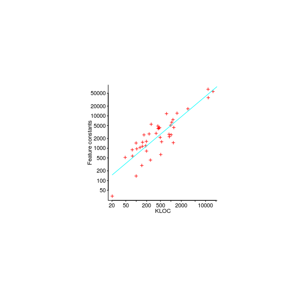
Figure 366. Cumulative percentage of configuration options impacting a given number of source files in the Linux kernel. Data kindly provided by Ziegler Ziegler_16. Github--Local

Figure 367. Density plot of the number of files containing code involved in supporting distinct options in four versions of Google Chrome. Data from Rahman et al Rahman_19. Github--Local

Figure 368. Number of selection-statements having a given maximum nesting level; fitted regression line has the form: $\mathit{num{_}selection}\propto e^{-0.7\mathit{nesting} }$. Data from Jones Jones_05a. Github--Local

Figure 369. Fraction of a project’s token sequences, containing a given number of tokens, that appear more than once in the projects' Java source (for 2,637 projects); the yellow line has the form: $\mathit{fraction}\propto a-b*\log(\mathit{seq{_}len} )$, where$a$ and $b$ are fitted constants. Data from Lin et al Lin_17. Github--Local

Figure 370. Number of Python source files containing a given number of SLOC; all files, and with duplicates removed. Data from Lopes et al Lopes_17. Github--Local

Figure 371. Number of reintroduced line sequences having a given difference in revision number between deletion and reintroduction (upper), and number of reintroduced line sequences containing a given number of lines (lower); the fitted regression lines have the form: $\mathit{Occurrence}\propto \mathit{NumLines}^{-1.4}e^{0.1\log(\mathit{NumLines})^2}$ and $\mathit{Occurrences}\propto \mathit{NumLines}^{-1.7}$. Data kindly provided by Kamiya Kamiya_11. Github--Local

Figure 372. The Berlin and Kay Berlin_69 language color hierarchy. The presence of any color term in a language implies the existence, in that language, of all terms below it. Papuan Dani has two terms (black and white), while Russian has eleven (Russian may also be an exception in that it has two terms for blue.) Github--Local

Figure 373. Mean compatibility of 50 applications to 11 versions of Python, over time. Data from Malloy et al Malloy_17. Github--Local

Figure 374. Cumulative number of developers who have committed Java source making use of particular new feature added to the language. Data from Dyer et al Dyer_14. Github--Local

Figure 375. Number of reads and writes to the same variable, for 3,315 variables occupying various amounts of storage, made during the execution of the Mediabench suite; grey line shows where number of writes equals number of reads. Data kindly provided by Caspi Caspi_00. Github--Local

Figure 376. Autocorrelation function of the argument values passed to the Bessel function j0. Data kindly provided by Suresh Suresh_15. Github--Local

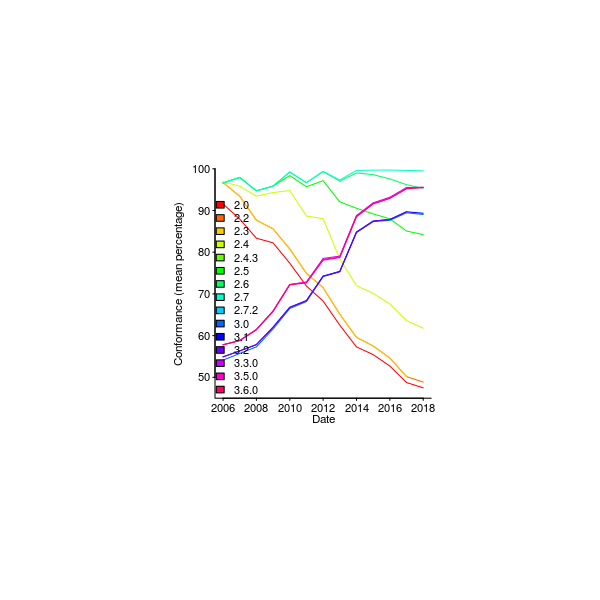
Figure 377. The number of dynamic statements, LOC and methods against total number of those constructs appearing in 28 Ruby programs; lines are power law regression fits. Data from Rodrigues et al Rodrigues_18. Github--Local

Figure 378. Total if-statements against if-statements whose condition involves a null check, in each of 800 Java projects; regression line fitted has the form: $\mathit{null{_}checks}\propto \mathit{Conditionals}$. Data kindly provided by Osman Osman_16. Github--Local

Figure 379. Percentage of conditional expressions, in 63 Java programs, containing a given number of clauses; one fitted regression model has the form: $\mathit{Num{_}conditions}\propto e^{ \mathit{Num{_}predicates}\times(\log(\mathit{SLOC})-0.6\log(\mathit{Files})-11)}$, where each variable is the total for a program’s source. Data from Durelli et al Durelli_16. Github--Local

Figure 380. Number of try blocks whose code might raise a given number of exceptions; fitted regression models have the form: (lower) $\mathit{Num{_}tryBlocks}\propto \mathit{Possible{_}exceptions}^{-0.22}$ and (upper) $\mathit{Num{_}tryBlocks}\propto 7300 e^{-1.4\mathit{Possible{_}exceptions} } +1100 e^{-0.21\mathit{Possible{_}exceptions} }$. Data from de Pádua et al de_Padua_17. Github--Local

Figure 381. Yearly occurrence of number words (e.g., "one", "twenty-two"), averaged over each year since 1960, in Google’s book data for three languages. Data kindly provided by Piantadosi Piantadosi_14. Github--Local

Figure 382. Percentage occurrence of the most significant digit of floating-point, integer and hexadecimal literals in C source code. Data from Jones Jones_05a. Github--Local

Figure 383. Number of C functions contains a given number of references to the same variable (upper), and a given number of references to all variables (lower); reads are full lines, writes dashed lines, colors indicate variable’s visibility. Data from Jones Jones_05a. Github--Local

Figure 384. Number of functions defined with a given number of parameters in the C source of four projects; solid lines function body did not access global variables, dashed lines function body accessed global variables. Data from Gonzaga Gonzaga_15. Github--Local

Figure 385. Sequences of methods, from java.lang.StringBuilder, called on the same object; based on 3,418 Jar files. Data from Mendez et al Mendez_13. Github--Local

Figure 386. For each Java class, in 3,418 jar files, the number of method sequences containing a given number of calls (red), and the number of uses of each sequence (blue). Data from Mendez et al Mendez_13. Github--Local

Figure 387. Number of distinct API methods called in 1,435 Java projects containing a given number of method calls; the line is a fitted regression model of the form: $\mathit{unique}\propto \mathit{calls}^{0.78}$. Data from Lämmel et al Lammel_11. Github--Local

Figure 388. Number of function calls, against corresponding number of calls containing callbacks and anonymous callbacks, in 130 Javascript programs; lines are fitted regression models of the form: $\mathit{allCallbacks}\propto \mathit{allCalls}^{0.86}$ and $\mathit{anonCallbacks}\propto \mathit{allCalls}^{0.8}$, respectively. Data from Gallaba et al Gallaba_15. Github--Local

Figure 389. Number of global variables against lines of code over 48 releases of three systems written in C. Data kindly provided by Neamtiu Neamtiu_05. Github--Local

Figure 390. Jittered number of data and operation extensions to 1,560 Smalltalk class hierarchies containing both kinds of extension; regression line has the form: $\log(\mathit{Data{_}extensions} )\propto \log(\mathit{Operation{_}extensions} )^2$. Data from Robbes et al Robbes_15. Github--Local

Figure 391. Number of C function definitions having a given number of parameters (red) and unused parameters (green); parameter fitted regression line has the form: $\mathit{functions}\propto e^{-0.67\mathit{parameters} }$. Data from Jones Jones_05a. Github--Local

Figure 392. "Worth estimate" for the kind of method activity attribute; see section. Data from Biegel et al Biegel_12. Github--Local

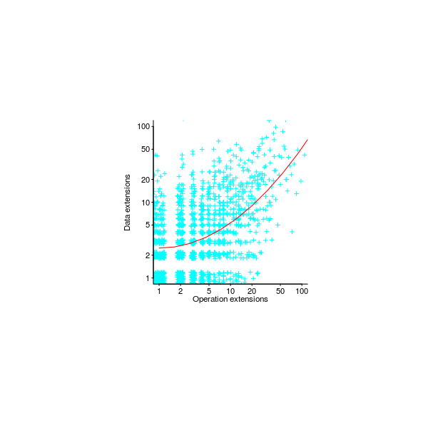
Figure 393. Dependencies between the Java packages in various versions of ANTLR. Data from Al-Mutawa Al-Mutawa_13. Github--Local

Figure 394. Fraction of source in 130 releases of Linux (x-axis) that originates in an earlier release (y-axis). Data extracted from png file kindly supplied by Matsushita Livieri_07. Github--Local

Figure 395. Number of functions in Evolution modified a given number of times (upper), and modified by a given number of different people (lower); red line is a fitted bi-exponential, green/blue lines are the individual exponentials. Data from Robles et al Robles_12a. Github--Local

Figure 396. Number of functions (in Evolution) modified a given number of times, broken down by number of authors; lines are a fitted regression model. Data from Robles et al Robles_12a. Github--Local

Figure 397. Density plot of the time interval, in hours, between each modification of the functions in Evolution and Apache. Data from Robles et al Robles_12a. Github--Local

Figure 398. Number of virus infections and UFO sighting, reported in 3,072 U.S. counties during 2010; the line is a fitted regression model of the form: $\mathit{virus{_}reports}\propto \mathit{UFO{_}reports}^{1.2}$. Data from Jacobs et al Jacobs_14. Github--Local

Figure 399. Data having values following various visual patterns, when plotted. Github--Local

Figure 400. Years of professional experience in a given language for experimental subjects. Data from Prechelt Prechelt_07. Github--Local

Figure 401. Total number of lines of C source, in .c and .h files, having a given length, i.e., containing a given number of characters (upper) and tokens (lower). Data from Jones Jones_05a. Github--Local

Figure 402. Various measurements of work performed implementing the same functionality, number of lines of Haskell and C implementing functionality, CFP (COSMIC function points; based on user manual) and length of formal specification. Data kindly provided by Staples Staples_13. Github--Local

Figure 403. Effort, in hours (log scale), spent in various development phases of projects written in Ada (blue) and Fortran (red). Data from Waligora et al Waligora_95. Github--Local

Figure 404. Performance of experts (e) and novices (n) in a test driven development experiment. Data from Muller et al Muller_07. Github--Local

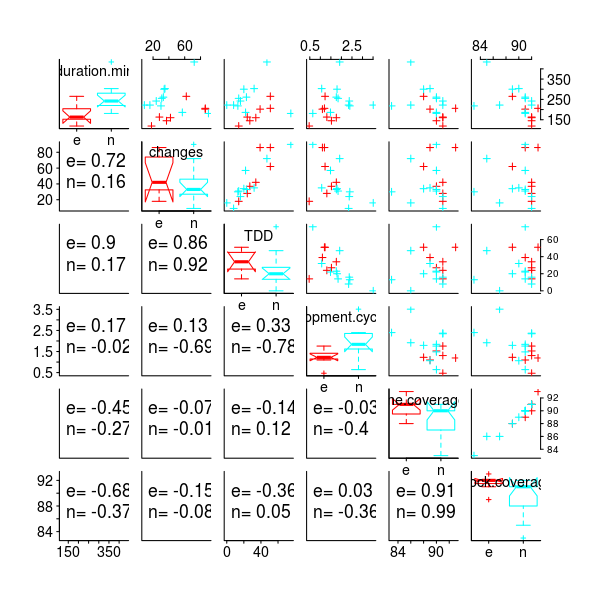
Figure 405. Correlations between pairs of attributes of 12,799 Github pull requests to the Homebrew repo, represented using numeric values and pie charts. Data from Gousios et al Gousios_14. Github--Local

Figure 406. Hierarchical cluster of correlation between pairs of attributes of 12,799 Github pull requests to the Homebrew repo. Data from Gousios et al Gousios_14. Github--Local

Figure 407. Number of computers having a given SPECint result; line is a loess fit. Data from SPEC SPEC_20. Github--Local

Figure 408. Effort invested in project definition (as percentage of original estimate) against cost overrun (as percentage of original estimate). Data extracted from Gruhl Gruhl_9x. Github--Local

Figure 409. Relative clock frequency of cpus when first launched (1970 == 1). Data from Danowitz et al Danowitz_12. Github--Local

Figure 410. Year and age at which survey respondents started contributing to FLOSS, i.e., made their first FLOSS contribution. Data from Robles et al Robles_14. Github--Local

Figure 411. Number of computers with a given SPECint result, summed within 13 equal width bins (upper) and kernel density plot (lower). Data from SPEC SPEC_20. Github--Local

Figure 412. Number of commits containing a given number of lines of code made when making various categories of changes to the Linux filesystem code (upper), and a density plot of the same data (lower). Data from Lu et al Lu_13. Github--Local

Figure 413. Histogram of the $\log$ of some measured quantity. Github--Local

Figure 414. Developer estimated effort against actual effort (in hours), for various maintenance tasks, e.g., adaptive, corrective and perfective; upper as-is, middle jittered values and lower size proportional to the $\log$ of the number measurements. Data from Hatton Hatton_07. Github--Local

Figure 415. Number of installations of Debian packages against the age of the package; middle plot was created by smoothScatter and lower plot by contour. Data from the "wheezy" version of the Ultimate Debian Database project UDD_14. Github--Local

Figure 416. Number of lines added to glibc each week. Data from González-Barahona et al Gonzalez-Barahona_14. Github--Local

Figure 417. Boxplot of time between a potential mistake in Eclipse being reported and the first response to the report; right plot is notched. Data from Breu et al Breu_10. Github--Local

Figure 418. Violin plot of time between bug being reported in Eclipse and first response to the report. Data from Breu et al Breu_10. Github--Local

Figure 419. Time taken for developers to debug various programs using batch processing or online (i.e., time-sharing) systems. Data kindly provided by Prechelt Prechelt_99a. Github--Local

Figure 420. Pairs of languages used together in the same GitHub project with connecting line width, color and transparency related to number of occurrences. Data kindly supplied by Bissyande Bissyande_13. Github--Local

Figure 421. References from one document to another in the Microsoft Server Protocol specifications. Data extracted by your author from the 2009 document release WSPP_15. Github--Local

Figure 422. Alluvial plot of relative prioritization order of selection and application of Github pull requests. Data from Gousios et al Gousios_15a. Github--Local

Figure 423. Intel Sandy Bridge L3 cache bandwidth in GB/s at various clock frequencies and using combinations of cores (0-3 denotes cores zero-through-three, 0,2,4 denotes the three cores: zero, two and four). Data from Schone et al Schone_12. Github--Local

Figure 424. Contour plot of number of sessions executed on a computer having a given processor speed and memory capacity. Data kindly provided by Thereska Thereska_10. Github--Local

Figure 425. Root source of 1,257 faults and where fixes were applied for 21 large safety critical applications. Data from Hamill et al Hamill_14. Github--Local

Figure 426. Ternary plots drawn with two possible visual aids for estimating the position of a point (red plus at x=0.1, y=0.35, z=0.55); axis names appear on the vertex opposite the axis they denote. Github--Local

Figure 427. Actual and estimated size ratio for bars and spheres, for each of the ten subjects (in different colors, with line from fitted regression model), with grey line showing where estimate equals actual. Data from Jansen et al Jansen_16. Github--Local

Figure 428. Earth relative positions of NASA’s Orbview-2 spacecraft when it experienced a single event upset (in blue) on 12 July 2000. Data kindly provided by LaBel Poivey_03. Github--Local

Figure 429. Estimated market share of Android devices by brand and product, based on downloads from 682,000 unique devices in 2015. Data from OpenSignal OpenSignal_15. Github--Local

Figure 430. Variables having a given number of read accesses, given 25, 50, 75 and 100 total accesses, calculated from running the weighted preferential attachment algorithm (red), the smoothed data (blue), and a fitted exponential (green). Github--Local

Figure 431. Throughput when running the SPEC SDM91 benchmark on a Sun SPARCcenter 2000 containing 8 CPUs, with the predictions from three fitted queuing models. Data from Gunther Gunther_05. Github--Local

Figure 432. Illustration of the difference in cognitive effort needed to locate points differing by shape or color (one is a serial search, while the other operates in parallel). Github--Local

Figure 433. The three, seven and twelve color palettes returned by calls to the diverge_hcl, sequential_hcl, rainbow_hcl and rainbow functions. Github--Local

Figure 434. Percentage share of Android market by successive Android releases, by individual version (top) and by date (lower); pastell colors on left and bold on right. Data from Villard Villard_15. Github--Local

Figure 435. Input case on which a failure occurred, for a total of 500,000 inputs; plotted using a linear (upper) and logarithmic (lower) x-axis. Data from Dunham et al Dunham_86. Github--Local

Figure 436. Example of U-shape created when y-axis values are a ratio calculated from x-axis values. Github--Local

Figure 437. Mean time to fail for systems of various sizes (measured in lines of code); linear y-axis left, log y-axis right. Data extracted from Figure 8.3 of Putnam et al Putnam_92. Github--Local

Figure 438. What’s up doc? Perhaps, not the expected pattern in the data. Equations from White White_12. Github--Local

Figure 439. Alternative representation of numeric values in table. Data from Scott Scott_16. Github--Local

Figure 440. Probability that three (red) or four (blue) consecutive false positive warnings occur in some total number of warnings (false positive rate appears on the line). Github--Local

Figure 441. Number of subjects rating more than eight jokes, with fitted bi-exponential model; line is a fitted regression model of the form: $\mathit{Subjects}\propto 4200 e^{-0.09\mathit{Jokes} } +650 e^{-0.02\mathit{Jokes} }$. Data from Goldberg et al Goldberg_01. Github--Local

Figure 442. The relationship between words for tracts of trees in various languages. The interpretation given to words (boundary indicated by the zigzags) in one language may overlap that given in other languages. Adapted from DiMarco et al DiMarco_93. Github--Local

Figure 443. Relationships between commonly used discrete and continuous probability distributions.

Figure 444. Shapes of commonly encountered discrete probability distributions (upper to lower: Uniform, Geometric, Binomial and Poisson). Github--Local

Figure 445. Cumulative density plots of the discrete probability distributions in figure. Github--Local

Figure 446. Commonly encountered continuous probability distributions (upper to lower: Uniform, Exponential, Normal, beta). Github--Local

Figure 447. Samples of randomly selected values drawn from the same normal distribution (left: 100 points in each sample, right 1,000 points in each sample). Github--Local

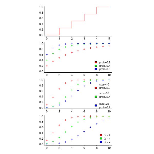
Figure 448. Reading rate for text printed using a serif (blue) and sans-serif (red) font, data has been normalised and displayed as a density. Data from Veytsman et al Veytsman_12. Github--Local

Figure 449. Probability, with p-value < 0.05, that shapiro.test correctly reports that samples drawn from various distributions are not drawn from a Normal distribution, and probability of an incorrect report when the sample is drawn from a Normal distribution; 1,000 replications for each sample size. Github--Local

Figure 450. Number of conditionally compiled code sequences dependent on a given number of feature macros (red overwritten by blue: Linux, blue: FreeBSD). Data from Berger et al Berger_10. Github--Local

Figure 451. Percentage occurrence of statements (x-axis) for each of 100 or so C, C++ and Java programs (colored lines, figure it out or look at the code), plotted as a density on the y-axis. Data from Zhu et al Zhu_15. Github--Local

Figure 452. A Cullen and Frey graph for the $3n+1$ program length data. Data kindly provided by van der Meulen van_der_Meulen_07. Github--Local

Figure 453. Number of 3n+1 programs containing a given number of lines, with four distributions fitted to this data. Data kindly provided by van der Meulen van_der_Meulen_07. Github--Local

Figure 454. A zero-truncated Negative Binomial distribution fitted to the number of features whose implementation took a given number of elapsed workdays; first 650 days used. Data kindly provided by 7digital 7Digital_12. Github--Local

Figure 455. Density plot of MPI micro-benchmark runtime performance for calls to MPI_Allreduce with 1,000 Bytes (left curve) and to MPI_Scan with 10,000 Bytes (right curve). Data kindly supplied by Hunold Hunold_14. Github--Local

Figure 456. Mixture model fitted by the normalmixEM function to the performance data from calls to MPI_Allreduce. Data kindly supplied by Hunold Hunold_14. Github--Local

Figure 457. Density plots of accesses to one article on Slashdot, in minutes since its publication. The distinct Normal distributions (colored and fitted to the log of the data) contained in the mixture models fitted by the REBMIX (upper) and normalmixEM (lower) functions. Data kindly supplied by Kaltenbrunner Kaltenbrunner_07. Github--Local

Figure 458. Cumulative probability distribution of files size (red) and of number of bytes occupied in a file system (blue). Data from Irlam Irlam_93. Github--Local

Figure 459. Graph of available state transitions for Alaris volumetric infusion pump (the button presses that cause transitions between states are not shown). Data kindly supplied by Oladimeji Oladimeji_08. Github--Local

Figure 460. Discrete-time Markov chain for created/modified/deleted status of Linux kernel files at each major release from versions 2.6.0 to 2.6.39. Data from Tarasov Tarasov_12. Github--Local

Figure 461. Directed graph of emails between FreeBSD and OpenBSD developers, plus a few people involved in both discussions, with developers who sent/received less than four emails removed. Data from Canfora et al Canfora_11. Github--Local

Figure 462. Expected probability of a single instance (y-axis) against the probability of a measured struct type having grouped member types (x-axis); when both probabilities are the same points will be along the blue line. Data from Jones Jones_09b. Github--Local

Figure 463. Example of a sample drawn from a population. Github--Local

Figure 464. Date of introduction of a cpu against its commercial lifetime; processors ceasing production in 2000 or 2010 would appear along one of the lines. Data from Culver Culver_10. Github--Local

Figure 465. A population of items having one of three colors, along with samples of the three strata (imperfect item selection introduces noise in the samples). Github--Local

Figure 466. Power consumed by three SERT benchmark programs at various levels of system load; crosses at 2% load intervals, lines based on 10% load intervals. Data kindly provided by Kistowski Kistowski_15. Github--Local

Figure 467. The four related quantities in the design of experiments; given three, the fourth can be calculated. Github--Local

Figure 468. Examples of the impact of population prevalence, statistical power and p-value on number of false positives and false negatives. Github--Local

Figure 469. Visualization of Cohen’s $d$ for two normal distributions having different means and the same standard deviation (two left), and different mean and standard deviations (two right). Github--Local

Figure 470. Distribution of 4,000 sample means, for two sample sizes, drawn from exponential (upper), lognormal (center) and Pareto (lower) distributions, vertical lines are 95% confidence bounds. The blue curve is the Normal distribution, predicted by theory. Github--Local

Figure 471. Mean (red) and standard deviation (brown line for each sample; not symmetrical because of log scaling) of samples of 3 items drawn from a population of 1,000 items (whose mean shown by blue line and standard deviation by green lines). Data kindly provided by Chen Chen_12. Github--Local

Figure 472. Density plot of mean of samples containing 3 or 12 items randomly selected from a data set of 1,000 items; process repeated 1,000 times for each sample size. Data kindly provided by Chen Chen_12. Github--Local

Figure 473. Number of commits to glibc for each day of the week, for the years from 1991 to 2012. Data from González-Barahona et al Gonzalez-Barahona_14. Github--Local

Figure 474. The impact of differences in mean and standard deviation on the overlap between two populations ($\alpha$: probability of making a false positive error, and $\beta$: probability of making a false negative error). Github--Local

Figure 475. Power analysis (50 and 10 runs at various p-values) of detecting a difference between two runs having a binomial distribution (runs needed to achieve power=0.8 at various p-values). Github--Local

Figure 476. The statistical power of detecting that a difference exists between the mean values of samples of various sizes drawn from two populations; actual mean difference between samples adjacent to colored line. Github--Local

Figure 477. A Normal distribution with mean=4 and variance=8 and a Chi-squared distribution with four degrees of freedom having the same mean and variance (the vertical lines are at the distributions' median value). Github--Local

Figure 478. Density plot of execution time of 1,000 input data sets, with lines marking the mean, median and mode. Data kindly supplied by Chen Chen_12. Github--Local

Figure 479. Impact of serial correlation, AR(1) in this example, on the calculated mean (upper) and standard deviation (lower) of a sample (the legends specify the amount of serial correlation). Github--Local

Figure 480. Number of sample median (upper) and mean (lower) values for 1,000 samples drawn from a binomial distribution. Github--Local

Figure 481. Density plot of two samples; samples either drawn from a Normal distribution or a Contaminated Normal distribution (i.e., values drawn from two normal distributions, with 10% of values drawn from a distribution having a standard deviation five times greater than the other); the lines bounding the 95% quartile identify the color used for each plot. Github--Local

Figure 482. Number of papers reporting a p-value equal to a given value; lines are a fitted segmented regression model (four segments were specified). Data from Head et al Head_15. Github--Local

Figure 483. Regression model (red line; pvalue=0.02) fitted to the number of correct/false security code review reports made by 30 professionals; blue lines are 95% confidence intervals. Data from Edmundson et al Edmundson_13. Github--Local

Figure 484. Bootstrapped regression lines fitted to random samples of the number of correct/false security code review reports made by 30 professionals. Data from Edmundson et al Edmundson_13. Github--Local

Figure 485. Kernel density plot, with 95% confidence interval, of the number of computers having the same SPECint result. Data from SPEC SPEC_20. Github--Local

Figure 486. One and two-sided significance testing. Github--Local

Figure 487. Number of Reflection benchmark results achieving a given score, reported for GTX 970 cards from three third-party manufacturers. Data extracted from UserBenchmark.com. Github--Local

Figure 488. Density plots of project bids submitted by companies before/after seeing a requirements document. Data from Jørgensen et al Jorgensen_04c. Github--Local

Figure 489. Density plot of task implementation estimates: with no instructions (red) and with instruction on what to do (blue). Data from Jørgensen el al Jorgensen_04. Github--Local

Figure 490. Examples of correlation between samples of two value pairs, plotted on x- and y-axis. Github--Local

Figure 491. Number of software faults having a given consequence, based on an analysis of faults in Cassandra. Data from Gunawi et al Gunawi_14. Github--Local

Figure 492. Relationship between data characteristics (edge labels) and applicable techniques (node labels) for building regression models.

Figure 493. Total lines of source code in FreeBSD by days elapsed since the project started (in 1993). Data from Herraiz Herraiz_08. Github--Local

Figure 494. Estimated cost and duration of 73 large Dutch federal IT projects, along with fitted model and 95% confidence intervals (green for the bounds of the fitted line and blue for the bounds of any new measurements). Data from Kampstra et al Kampstra_09. Github--Local

Figure 495. Number of updates and fixes in each Linux release between version 2.6.11 and 3.2. Data from Corbet et al Corbet_12. Github--Local

Figure 496. Number of commits made, and the number of contributing developers for Linux versions 2.6.0 to 3.12. The blue line in the right plot is the regression model fitted by switching the x/y values. Data from Kroah-Hartman Kroah-Hartman_14. Github--Local

Figure 497. Effort/Size of various projects and regression lines fitted using Effort as the response variable (red, with green 95% confidence intervals) and Size as the response variable (blue). Data from Jørgensen et al Jorgensen_03. Github--Local

Figure 498. Lines of code in every initial release (i.e., excluding bug-fix versions of a release) of the Linux kernel since version 1.0, along with fitted straight line (upper) and quadratic (lower) regression models. Data from Israeli et al Israeli_10. Github--Local

Figure 499. Actual (left of vertical line), and predicted (right of vertical line) total lines of code in Linux at a given number of days since the release of version 1.0, derived from a regression model built from fitting a cubic polynomial to the data (dashed lines are 95% confidence bounds). Data from Israeli et al Israeli_10. Github--Local

Figure 500. Number of classes in the Groovy compiler at each release, in days since version 1.0. Data From Vasa Vasa_10. Github--Local

Figure 501. For each distinct language, the number of lines committed on Github, and the number of questions tagged with that language. Data from Kunst Kunst_13. Github--Local

Figure 502. Percentage of vulnerabilities detected by developers who have worked a given number of years in security. Data extracted from Edmundson et al Edmundson_13. Github--Local

Figure 503. Hours to develop software for 29 embedded consumer products, and the amount of code they contain, with fitted regression model and loess fit (yellow). Data from Fenton el al Fenton_08. Github--Local

Figure 504. Points remaining after removal of overly influential observations, repeatedly applying Cook’s distance and Studentized residuals. Data from Fenton el al Fenton_08. Github--Local

Figure 505. influenceIndexPlot for the model having the fitted line shown in figure; top three data points highlighted. Data from Fenton el al Fenton_08. Github--Local

Figure 506. Points remaining after removal of overly influential observations, also taking into account the Bonferroni p-value of the Studentized residuals; the line shows the fitted model and 95% confidence interval (loess fit in yellow). Data from Fenton el al Fenton_08. Github--Local

Figure 507. Number of medical devices reported recalled by the US Food and Drug Administration, in two week bins; fitted straight line and confidence bounds, with loess fit (yellow). Data from Alemzadeh et al Alemzadeh_13. Github--Local

Figure 508. influenceIndexPlot of data from Alemzadeh et al Alemzadeh_13. Github--Local

Figure 509. Two fitted straight lines and confidence intervals, one up to the end of 2010 and one after 2010. Data from Alemzadeh et al Alemzadeh_13. Github--Local

Figure 510. Results from various studies of software requirements function points counted using COSMIC and FPA; lines are loess fits to studies based on industry and academic counters. Data from Amiri et al Amiri_11. Github--Local

Figure 511. Five different equations fitted to the Embedded subset of the COCOMO 81 data before influential observation removal (upper) and after influential observation removal (lower). Data from Boehm Boehm_81. Github--Local

Figure 512. Anscombe data sets with Pearson correlation coefficient, mean, standard deviation, and line fitted using linear regression. Data from Anscombe Anscombe_73. Github--Local

Figure 513. Residual of the straight line fit to the Linux growth data analysed in figure. Data from Israeli et al Israeli_10. Github--Local

Figure 514. Array element assignment benchmark compiled with gcc using the O0 (upper) and O3 (lower) options (measurements were grouped into runs of 2,000 executions). Data from Flater et al Flater_13. Github--Local

Figure 515. Number of installations of Debian packages against the age of the package, plus fitted model and loess fit. Data from the "wheezy" version of the Ultimate Debian Database project UDD_14. Github--Local

Figure 516. Change-points detected by cpt.mean, upper using method="AMOC" and lower using method="PELT". Data from Alemzadeh et al Alemzadeh_13. Github--Local

Figure 517. Fitted regression model (blue) and adjusted model with one change-point (red). Data from Alemzadeh et al Alemzadeh_13. Github--Local

Figure 518. Monthly unit sales (in millions) of 4-bit microprocessors. Data kindly supplied by Turley Turley_02. Github--Local

Figure 519. Quadratic relationship with various amounts of added noise, fitted using a quadratic and exponential model. Github--Local

Figure 520. Author workload against number of activity types per author (upper) and ratio test (lower). Data from Vasilescu et al Vasilescu_12. Github--Local

Figure 521. Fitted regression line to points (in red) and 3-D representation of assumed Normal distribution for measurement error. Github--Local

Figure 522. Number of vulnerabilities detected by professional developers with web security review experience; upper: technically correct plot of model fitted using a Poisson distribution, lower: simpler to interpret curve representation of fitted regression models assuming measurement error has a Poisson distribution (continuous lines), or a Normal distribution (dashed lines). Data extracted from Edmundson Edmundson_13. Github--Local

Figure 523. Number of functions containing a given number of break statements and a fitted Negative Binomial distribution. Data from Jones Jones_05a. Github--Local

Figure 524. Number of APIs used in Java programs containing a given number of LOC; lines are fitted models based on a zero-truncated Poisson (red), Poisson and Normal distributions (blue, with confidence intervals in green), yellow line is loess fit. Data from Starek Starek_10. Github--Local

Figure 525. Code review meeting duration for a given number of non-comment lines of code; fitted regression model, assuming errors have a Gamma distribution (red, with confidence interval in blue), or a Normal distribution (green). Data from Porter et al Porter_98. Github--Local

Figure 526. Annual development cost and lines of Fortran code delivered to the US Air Force between 1962 and 1984; lines show fitted regression models (red: log transformed, blue: using a log link function) before(solid)/after(dotted) outlier removed (circled in red). Data extracted from NeSmith NeSmith_86. Github--Local

Figure 527. Maintenance task effort and lines of code added+updated, with fitted regression model (red), and SIMEX adjusted for estimated 10% error (blue). Data from Jørgensen Jorgensen_95. Github--Local

Figure 528. Regression modeling 0/1 data with a straight line and a logistic equation. Github--Local

Figure 529. ROC curve for the data listed in table. Github--Local

Figure 530. Probability of subject response being within a given percentage interval, based on their response to question q31. Data kindly provided by Luthiger Luthiger_07 . Github--Local

Figure 531. Percentage of mutants killed at various percentage of path coverage for 300 or so Java projects; fitted Beta regression (red), with 95% confidence intervals (blue) and glm (green) regression models. Data from Gopinath et al Gopinath_14. Github--Local

Figure 532. SPECint 2006 performance results for processors running at various clock rates, memory chip frequencies and processor family. Data from SPEC SPEC_20. Github--Local

Figure 533. Component+residual plots for three explanatory variables in a fitted SPECint model. Github--Local

Figure 534. Individual contribution of each explanatory variable to the response variable in a quadratic model of SPECint performance. Github--Local

Figure 535. Contour map of Result values predicted by a fitted model of SPECint performance, over range of Processor.MHz and mem_rate values. Github--Local

Figure 536. Estimated and actual effort broken down by communication frequency, along with individually fitted straight lines. Data from Moløkken-Østvold et al Molokken_Ostvold_07. Github--Local

Figure 537. Illustration of the shared and non-shared contributions made by two explanatory variables to the response variable Y. Github--Local

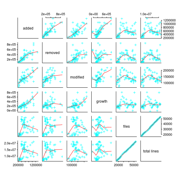
Figure 538. pairs plot of lines added/modified/removed, growth and number of files and total lines in versions 2.6.0 through 3.9 of the Linux kernel. Data from Kroah-Hartman Kroah-Hartman_14. Github--Local

Figure 539. Example plots of functions listed in table. These equations can be inverted, so they start high and go down. Github--Local

Figure 540. Time to execute a computational biology program on systems containing processors with various L2 cache sizes. Data kindly provided by Hazelhurst Hazelhurst_10. Github--Local

Figure 541. A logistic equation fitted to the lines of code in every non-bugfix release of the Linux kernel since version 1.0. Data from Israeli et al Israeli_10. Github--Local

Figure 542. Predictions made by logistic equations fitted to Linux SLOC data, using subsets of data up to 2900, 3650, 4200 number of days and all days since the release of version 1.0. Data from Israeli et al Israeli_10. Github--Local

Figure 543. Increase in areal density of hard disks entering production over time. Data from Grochowski et al Grochowski_12. Github--Local

Figure 544. Lines of code in the GNU C library against days since 1 January 1990. Data from González-Barahona Gonzalez-Barahona_14. Github--Local

Figure 545. Number of failing programs caused by unique fault experiences in gcc (upper) and SpiderMonkey (lower). Fitted model in green, with two exponential components in red and blue. Data kindly provided by Chen Chen_13. Github--Local

Figure 546. Power law (red) and exponential (blue) fits to feature macro usage in 20 systems written in C; fail to reject p-value for 20 systems is 0.64. Data from Queiroz et al Queiroz_17. Github--Local

Figure 547. Power consumption of six different Intel Core i5-540M processors running at various frequencies; colored lines denote fitted regression models for each processor. Data from Balaji et al Balaji_12. Github--Local

Figure 548. Example showing the three ways of structuring a mixed-effects model, i.e., different intersections/same slope (upper), same intersection/different slopes (middle) and different intersections/slopes (lower). Github--Local

Figure 549. Confidence intervals, 95%, for first (upper) and second (lower) call to lmer; within-subject intercepts (left column) and slopes (right column) for the mixed-effects models in the adjacent code. Github--Local

Figure 550. Number of files and lines of code in 3,782 projects hosted on Sourceforge; lines are 95%, 50% and 5% quantile regression fits. Data from Herraiz Herraiz_08. Github--Local

Figure 551. Expected maximum number of daily emails to the C++ lib email list expected to occur within a given period of months, with 95% confidence intervals; a GEP fitted model (corresponding plot function does not provide any user interface options). Data kindly extracted from the WG21 mailing list archive by Roger Orr. Github--Local

Figure 552. The three components of the hourly rate of commits, during a week, to the Linux kernel source tree; components extracted from the time series by stl. Data from Eyolfson et al Eyolfson_11. Github--Local

Figure 553. Autocorrelation of number of defects found on a given day, for development project C. Data kindly provided by Buettner Buettner_08. Github--Local

Figure 554. Autocorrelation of two AR models (upper plots) and two MA models (lower plots); the same models are used in figure. Github--Local

Figure 555. Partial autocorrelation of two AR models (upper plots) and two MA models (lower plots); the same models are used in figure. Github--Local

Figure 556. Autocorrelation of indentation of source code written in various languages. Data from Hindle et al Hindle_08. Github--Local

Figure 557. Number of features started for each day and fitted regression trend line (upper) and number of features after subtracting the trend (lower). Data kindly supplied by 7Digital 7Digital_12. Github--Local

Figure 558. Autocorrelation (upper) and partial autocorrelation (lower) of the number of features started on a given day (after differencing the log transformed data), over the entire period of the 7digital data. Data kindly supplied by 7Digital 7Digital_12. Github--Local

Figure 559. Monthly sales of spreadsheets in the UK, starting January 1987, with 12-months of sales predictions (shaded light blue are 80% confidence intervals, grey shaded 95%). Data from Givon et al Givon_95. Github--Local

Figure 560. Time series whose values are uncorrelated (upper), but whose squared values are correlated (lower); see code for generation process. Github--Local

Figure 561. The number of commits per week to Linux kernel source and its Kconfig files. Data kindly provided by Lotufo Lotufo_10. Github--Local

Figure 562. Cross correlation of feature release “size” (upper non-bugfix releases, lower all releases) and date when bugs are prioritised. Data kindly supplied by 7Digital 7Digital_12. Github--Local

Figure 563. Cross-correlation of source lines added/deleted per week to the glibc library. Data from González-Barahona Gonzalez-Barahona_14. Github--Local

Figure 564. The number of commits per week to Linux kernel source and its Kconfig files, during the last half of 2005. Data kindly provided by Lotufo Lotufo_10. Github--Local

Figure 565. Visualization of alignment between lines of code, in NetBSD’s (blue) and FreeBSD’s (red) first 100 weeks. Data from Herraiz Herraiz_08 Github--Local

Figure 566. Effort distribution (person hours) over the eight main tasks of a development project at Rolls-Royce and a hierarchical clustering of each task effort time series based on pair-wise correlation and Euclidean distance metrics. Data extracted from Powell Powell_01. Github--Local

Figure 567. Two commonly used hazard functions; Weibull is monotonic (always increases, decreases or remains the same, depending on the equation coefficients), and Lognormal which can increase and then decrease. Github--Local

Figure 568. Observation period of study, with events inside and outside the study period. Github--Local

Figure 569. The Kaplan-Meier curve for survivability of new releases: (blue) ETPs using only official APIs, (blue) ETPs calling internal APIs (red); dotted lines are 95% confidence intervals. Data from Businge Businge_13. Github--Local

Figure 570. The Kaplan-Meier curve for survivability of ETPs ability to be built using SDK released in subsequent years: (blue) ETPs using only official APIs, (red) ETPs calling internal APIs; dotted lines are 95% confidence intervals. Data from Businge Businge_13. Github--Local

Figure 571. Kaplan-Meier curves for time-to-release a patch for a reported vulnerability, with private, public, and private then public notification. Data from Arora et al Arora_10. Github--Local

Figure 572. Cumulative number of issues reported and closed, and issue survival curves for three intervals. Data from Lunesu Lunesu_13. Github--Local

Figure 573. Cumulative incidence curves for problems reported by the splint tool in Samba and Squid (time is measured in number of snapshot releases). Data from Di Penta et al Di_penta_09. Github--Local

Figure 574. Rose diagram of number of commits in each 3-hour period of a day for Linux and FreeBSD. Data from Eyolfson et al Eyolfson_11. Github--Local

Figure 575. The Cartwright (red; dcarthwrite), wrapped Cauchy (green; dwrappedcauchy) and wrapped von Mises (blue; dvonmises) circular probability distributions for various values of their parameters. Github--Local

Figure 576. Asymmetric extended wrapped forms of the Cardioid (upper), von Mises (middle) and Cauchy (lower) probability distributions for various values of their parameters. Github--Local

Figure 577. Number of readers of author’s blog, whose birthday falls within a given month and who have worked on a compiler. Data from Jones Jones_12b. Github--Local

Figure 578. Number of commits (upper) and number of commits in which a fault was detected (lower) by hour of day of the commit, for Linux. Data from Eyolfson et al Eyolfson_14. Github--Local

Figure 579. Number of non-fault related commits, and commits related to fixing a reported fault, per hour for weekdays, for linux; with fitted models. Data from Eyolfson et al Eyolfson_14. Github--Local

Figure 580. Number of commits per hour for each weekday, fitted using $\cos(\ldots\cos\ldots)$ (upper), and $\cos(\ldots\cos+\sin\ldots)$ (lower), for Linux; in both cases the fitted fault model (red) has been rescaled to allow comparison. Data from Eyolfson et al Eyolfson_14. Github--Local

Figure 581. Lines of source against percentage test coverage achieved by both Human & Dynodroid tests, only by Dynodroid tests and only by Human tests, for each of the 50 applications. Data from Machiry et al Machiry_13. Github--Local

Figure 582. Ternary plot composed from source lines covered by both Human & Dynodroid tests, by only by Dynodroid tests and only by Human tests (measurements in blue); fitted regression line (green) and prediction points (red) for various total source lines (numeric values). Data from Machiry et al Machiry_13. Github--Local

Figure 583. Volume of unit sphere in 1 to 50 dimensions, e.g., sphere has volume $\frac43pi$ in three dimensions. Github--Local

Figure 584. Top levels of the decision tree fitted to the reopened fault data (overly long lines are names of people who reported and fixed the fault). Data from Shihab et al Shihab_10a. Github--Local

Figure 585. Unrooted tree denoting a phylogenetic tree estimated from the paired similarity of the corresponding source files contained in some releases of the major variants of BSD unix. Data kindly supplied by Kanda Kanda_15. Github--Local

Figure 586. A two-key plot of associating mining results; order indicates number of items in rules. Data from Fowkes et al Fowkes_16. Github--Local

Figure 587. A Bertin plot for items included in the same data structure as the item “Antibiotics used”, for each numbered subject, after reordering by seriate. Data from Jones Jones_09b. Github--Local

Figure 588. A visualization of the Robinson matrix based on number of times pairs of items co-occur in the same data structure (the closer to the diagonal the more often they occur together). Data from Jones Jones_09b. Github--Local

Figure 589. Relative ordering of binary operator precedence (i.e., value of $\beta$), and corresponding standard error, based on subject responses to binary operator precedence questions. Data from Jones Jones_06a. Github--Local

Figure 590. Fitted values of $\beta$ for access control (visibility) of method definitions within a Java class. Data from Biegel et al Biegel_12. Github--Local

Figure 591. Region populations and their connections: initial conditions used in Duggan’s Duggan_17 numerical solution of the Bass equation. Github--Local

Figure 592. Number of nodes in the Python call graphs built by four tools, broken down by number of nodes common to each tool. Data from Li Li_19. Github--Local

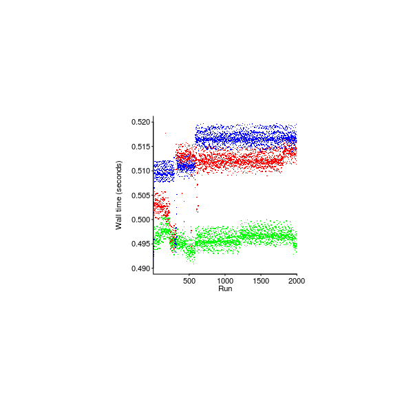
Figure 593. Time taken by 2,000 runs of a Javascript BinaryTree benchmark, with JIT enabled, on a quad-core Intel i7-4790; three colors are three iterations of the process: reboot machine, execute 2,000 runs. Data from Barrett et al Barrett_16. Github--Local

Figure 594. Time taken to transfer and multiply 2-dimensional matrices of various sizes on a GTX 480 GPU. Data kindly supplied by Gregg Gregg_11. Github--Local

Figure 595. Relative performance (y-axis) of libraries optimized to run on various processors (x-axis). Data from Bird Bird_10. Github--Local

Figure 596. Number of integer constants, appearing in the visible form of C source code, having the lexical form of a decimal-constant (the literal 0 is also included in this set) and hexadecimal-constant that have a given value. Data from Jones Jones_05a. Github--Local

Figure 597. A cube plot of three configuration factors and corresponding benchmark results (blue) from Memory table experiment. Data from Citron et al Citron_03b. Github--Local

Figure 598. Design plot showing the impact of each configuration factor on the performance of Memo table on benchmark performance. Data from Citron et al Citron_03b. Github--Local

Figure 599. Interaction plot showing how cint changes with size, for given values of mapping. Data from Citron et al Citron_03b. Github--Local

Figure 600. Half-normal plot of data from a Plackett and Burman design experiment. Data from Debnath et al Debnath_08. Github--Local

Figure 601. Performance and rental cost of early computers, with straight line fits for a few years. Data from Knight Knight_66. Github--Local

Figure 602. Feature size, in Silicon atoms, of microprocessors; line is a fitted regression of the form: $\mathit{Silicon{_}atoms}\propto e^{-0.17\mathit{Year} }$. Data from Danowitz et al Danowitz_12. Github--Local

Figure 603. Maximum number of records sorted in 1 minute and using 1 penny’s worth of system time (upper), and SPEC2006 integer benchmark results (lower, with loess fit). Data from Gray et al Gray_14 and SPEC SPEC_20. Github--Local

Figure 604. Mean time for an Intel IvyBridge to transition from a given frequency (colored lines) to another frequency (x-axis). Data kindly provided by Mazouz Mazouz_14. Github--Local

Figure 605. Total system power consumed when sorting 10, 20, 30, 40, 50 million integers (colored pluses), using Radix sort on the same processor running at different clock frequencies. Data from Götz et al Gotz_14. Github--Local

Figure 606. Power consumed by an Exynos-7420 A53 processor at various frequencies, and one to four cores under load, with fitted regression lines. Data kindly provided by Frumusanu Frumusanu_15. Github--Local

Figure 607. Power consumed by 10 Amtel SAM3U microcontrollers at various temperatures when sleeping or running. Data from Wanner et al Wanner_10. Github--Local

Figure 608. Time taken to execute the EP benchmark and clock frequency of 2,386 Intel processors, with a RAPL of 65 Watts. Data kindly provided by Rountree Marathe_17. Github--Local

Figure 609. Power spectrum of the electrical power consumed by the Botanica App executing on a BeagleBone Black running Android 4.2.2. Data from Saborido et al Saborido_15. Github--Local

Figure 610. Read bandwidth at various offsets for new disks sold in 2002 (upper) and 2006 (lower). Data kindly provided by Krevat Krevat_13. Github--Local

Figure 611. Average power consumed by one server’s CPU (four Pentium 4 Xeons; red) and memory (8 GB PC133 DIMMs; blue) running the SPEC CPU2006 benchmark (upper) and breakdown by system component when executing various programs. Data from Bircher Bircher_10. Github--Local

Figure 612. Time taken to find a unique item in arrays of various size, containing distinct items, using various search algorithms; grey lines are L1, L2 and L3 processor cache sizes. Data from Khuong et al Khuong_15. Github--Local

Figure 613. FFT benchmark executed 2,048 times followed by system reboot, repeated 10 times. Data kindly provided by from Kalibera_05. Github--Local

Figure 614. Percentage change, relative to no environment variables, in perlbench performance as characters are added to the environment. Data extracted from Mytkowicz et al Mytkowicz_08. Github--Local

Figure 615. Changes in SPEC CPU2006 performance caused by cache and memory bus contention, for one dual processor Intel Xeon E5345 system. Data kindly provided by Babka Babka_12. Github--Local

Figure 616. Execution time of 330.art_m, an OpenMP benchmark program, using different compilers, number of threads and setting of thread affinity. Data kindly provided by Mazouz Mazouz_13. Github--Local

Figure 617. Access times when walking through memory using three fixed stride patterns (i.e., 32, 64 and 128 bytes) on a quad-core Intel Xeon E5345; grey lines at one standard deviation. Data kindly provided by Babka Babka_09. Github--Local

Figure 618. Performance variation of programs from the Talos benchmark run on original OS and a stabilised OS. Data from Larres Larres_12. Github--Local

Figure 619. Operations per second of a file-sever mounted on one of ext2, ext3, rfs and xfs filesystems (same color for each filesystem) using various options. Data kindly supplied by Huang Zhou_12. Github--Local

Figure 620. Percentage change in SPEC number, relative to version 4.0.4, for 12 programs compiled using six different versions of gcc (compiling to 64-bits with the O3 option). Data from Makarow Makarow_14. Github--Local

Figure 621. Execution time of the xy file compressor, compiled using gcc using various optimization options, running on various systems (lines are mean execution time when compiled using each option). Data kindly supplied by Petkovich de_Oliveira_13. Github--Local

Figure 622. Execution time of Perlbench, part of the SPEC benchmark, on six systems, when linked in three different orders and address randomization on/off. Data kindly supplied by Reidemeister de_Oliveira_13. Github--Local

Figure 623. Ubench cpu performance on small (upper) and large (lower) EC2 instances, Europe in red and US in green. Data kindly provided by Dittrich Schad_10. Github--Local

Figure 624. Performance of PassMark memory benchmark on 783 Intel Core i7-3770K systems; line is fitted $\logit$ model. Data kindly supplied by Wren PassMark_14. Github--Local

Figure 625. Number of lines of code that 101 professional developers, with a given number of years experience, estimate they have written, lines are various regression fits. Data from Jones Jones_06aJones_08aJones_09b. Github--Local

Figure 626. Probability that a subject, having a given relative ability, will answer a question correctly: lines are for each question in a fitted Rasch model. Data from Dietrich et al Dietrich_14. Github--Local

Figure 627. Reported LOC and duration of 2,751 code reviews, for one company; reported reviews lasting less than 30 seconds (below green line), involving more than 2,000 LOC (to right of red line), processing at a rate greater than 1,500 LOC per hour (above blue line). Data extracted from Cohen et al Cohen_12. Github--Local

Figure 628. Screen height and width reported by 682,000 unique devices that downloaded an App from OpenSignal in 2015 (upper), reported measurements ordered so height always the larger value (lower). Data from OpenSignal OpenSignal_15. Github--Local

Figure 629. Number of reported vulnerabilities, per day, in the US National Vulnerability Database for 2003. Data from the National Vulnerability Database NVD_14. Github--Local

Figure 630. Estimated staff working on a project during each week; lines are a fitted loess model and 95% confidence bounds. Data from Buettner Buettner_08. Github--Local

Figure 631. Market share of Firefox version 3.0 fitted using loess regression with various values of the span option. Data from W3Counter W3Counter_14. Github--Local

Figure 632. Percentage occurrence of the first digit of hexadecimal numbers in C source and estimated from Google book data. Data from Jones Jones_05a and Michel et al Michel_11. Github--Local

Figure 633. Number of processes executing for a given amount of time, with measurements expressed using two and six significant digits. Data from Feitelson Feitelson_14. Github--Local

Figure 634. Plot produced by hello_world.R program. Github--Local

Figure 635. The unique bytes per window (256 bytes wide) of a pdf file. Github--Local